Single Analog Input – Continuous
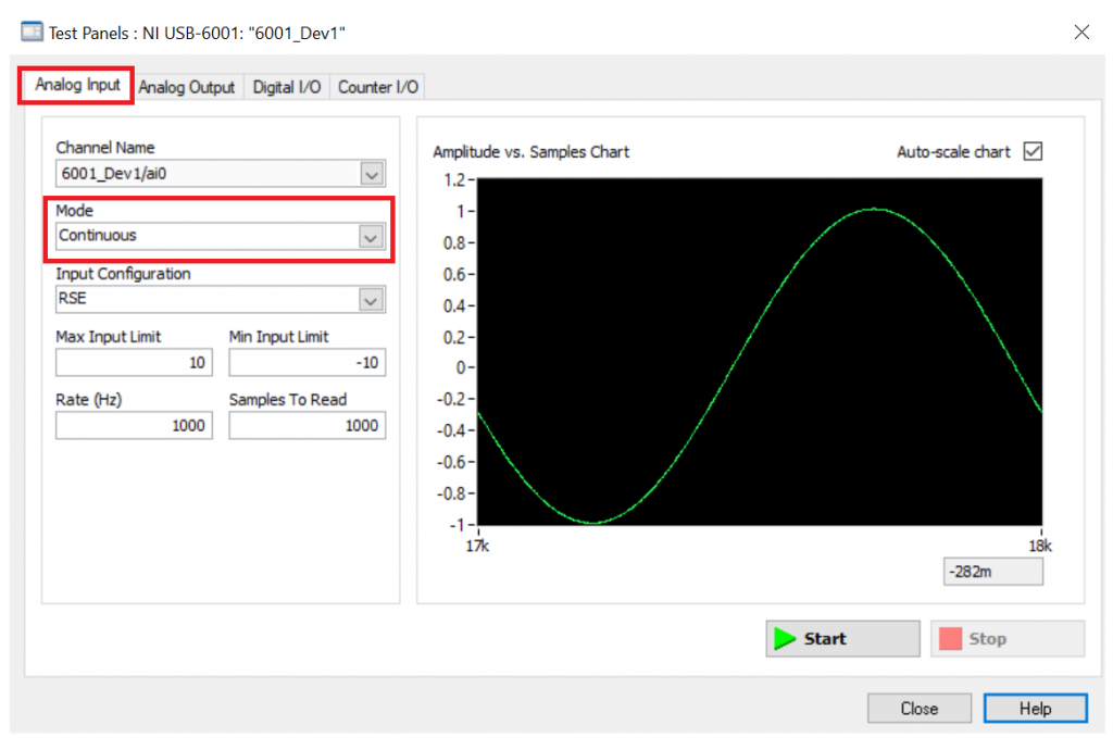
For this article I am going to show how to implement the continuous single analog input mode from the test panel NI-MAX software. I encourage to test this mode first using the NI-MAX software in order to get a better feeling what are the pros and cons of this mode before looking at the python examples.
Intro
The continuous mode can be used when the user wants to acquire analog values with faster rates and not lose any data while, for example, plotting data in real time.
The Rate and Samples to Read parameters are used to set the required amount of data and acquisition time accordingly.
I will present below python examples that shows the analog reading on a terminal, and on a Graphical User Interface (GUI), so you can use the code that works best for your needs.
In general, data acquisition programming with DAQmx involves the following steps:
- Create a Task and Virtual Channels
- Configure the Timing Parameters
- Start the Task
- Perform a Read operation from the DAQ
- Perform a Write operation to the DAQ
- Stop and Clear the Task.
Terminal
I start with the terminal code because it is the easiest to follow and the GUI code builds from this one. You have access to the full code under the Python Files section.
Start by including the nidaqmx library. Change the device_name variable according to the name of your device. Change ai0 to any other analog input that you would like to use.
import nidaqmx
from nidaqmx import constants
from nidaqmx.stream_readers import AnalogSingleChannelReader

import numpy as np

device_name = "6001_Dev1/ai0"

analog_task = None
The function ai_single_continuous() performs the steps to acquire data in continuous mode. It starts by creating the analog task using the nidaqmx.Task() function. After that, it parameterizes the analog channel, and sets the acquisition type to continuous mode. Since we set the acquisition to continuous mode, the NI-DAQmx will allocate a buffer to store the data at regular intervals. The function analog_task.register_every_n_samples_acquired_into_buffer_event() is used to register a callback function that the user can use to empty the buffer and process the acquired data respectively.
def ai_single_continuous():
    global analog_task

    #  Create Task
    # --------------
    analog_task = nidaqmx.Task()

    #  Create Virtual Channel - Analog Input
    # --------------------------------------
    analog_task.ai_channels.add_ai_voltage_chan(physical_channel=device_name,
                                                name_to_assign_to_channel="",
                                                terminal_config=constants.TerminalConfiguration.RSE,
                                                min_val=-10.0,
                                                max_val=10.0,
                                                units=constants.VoltageUnits.VOLTS,
                                                custom_scale_name=None)

    #  Sets the source of the Sample Clock, the rate of the Sample
    #  Clock, and the number of samples to acquire or generate.
    Fs = 1000.0  # Hz
    samples_per_channel = 1000
    analog_task.timing.cfg_samp_clk_timing(rate=Fs,
                                           source=None,
                                           active_edge=nidaqmx.constants.Edge.RISING,
                                           sample_mode=nidaqmx.constants.AcquisitionType.CONTINUOUS,
                                           samps_per_chan=samples_per_channel)

    # Register my_callback function
    analog_task.register_every_n_samples_acquired_into_buffer_event(samples_per_channel, my_callback)

    #  Start Task
    # -----------
    analog_task.start()

    #  Acquire Analog Value
    # ---------------------
    # my_callback function takes care of the analog acquisition

    input("")

    #  Stop and Clear Task
    # --------------------
    analog_task.stop()
    analog_task.close()
In this particular case, the callback function is very simple, it gets the data from the buffer and prints the result to the terminal.
def my_callback(task_handle, every_n_samples_event_type, number_of_samples, callback_data):
    global analog_task

    np_values = analog_task.read(number_of_samples_per_channel=nidaqmx.constants.READ_ALL_AVAILABLE,
                                 timeout=nidaqmx.constants.WAIT_INFINITELY)

    print("Sample Size: " + str(len(np_values)))
    print(np_values)

    return 0
Analog Input Configuration Functions
Change the parameters of the analog input virtual channel according to your application needs.
#  Create Virtual Channel - Analog Input
analog_task.ai_channels.add_ai_voltage_chan(
     physical_channel=device_name,
     name_to_assign_to_channel="",
     terminal_config=constants.TerminalConfiguration.RSE,
     min_val=-10.0,
     max_val=10.0,
     units=constants.VoltageUnits.VOLTS,
     custom_scale_name=None)
Change the sampling rate and number of samples per channel according to your application requirements.
#  Sets the source of the Sample Clock, the rate of the Sample
    #  Clock, and the number of samples to acquire or generate.
    Fs = 1000.0  # Hz
    samples_per_channel = 1000
    analog_task.timing.cfg_samp_clk_timing(rate=Fs,
                                           source=None,
                                           active_edge=nidaqmx.constants.Edge.RISING,
                                           sample_mode=nidaqmx.constants.AcquisitionType.CONTINUOUS,
                                           samps_per_chan=samples_per_channel)
Call ai_single_continuous() from the main function.
if __name__ == "__main__":
    ai_single_continuous()
Result
Let's do a simple test and set the sampling frequency (Fs) to 1kHz and the number of samples (samples_per_channel) to 1000, which means that we will acquire 1 second worth of data. Let's also set the function generator to generate a sinusoidal wave form at 1Hz. With this parameters we should be able to acquire one full cycle of the input waveform.
If you run the code, you will see that the code will display the acquired data on the terminal every 1 second. To stop the acquisition, press any key on the keyboard.
To validate that we are receiving the correct values, I copied the results from the terminal and use Octave Online to plot the data.
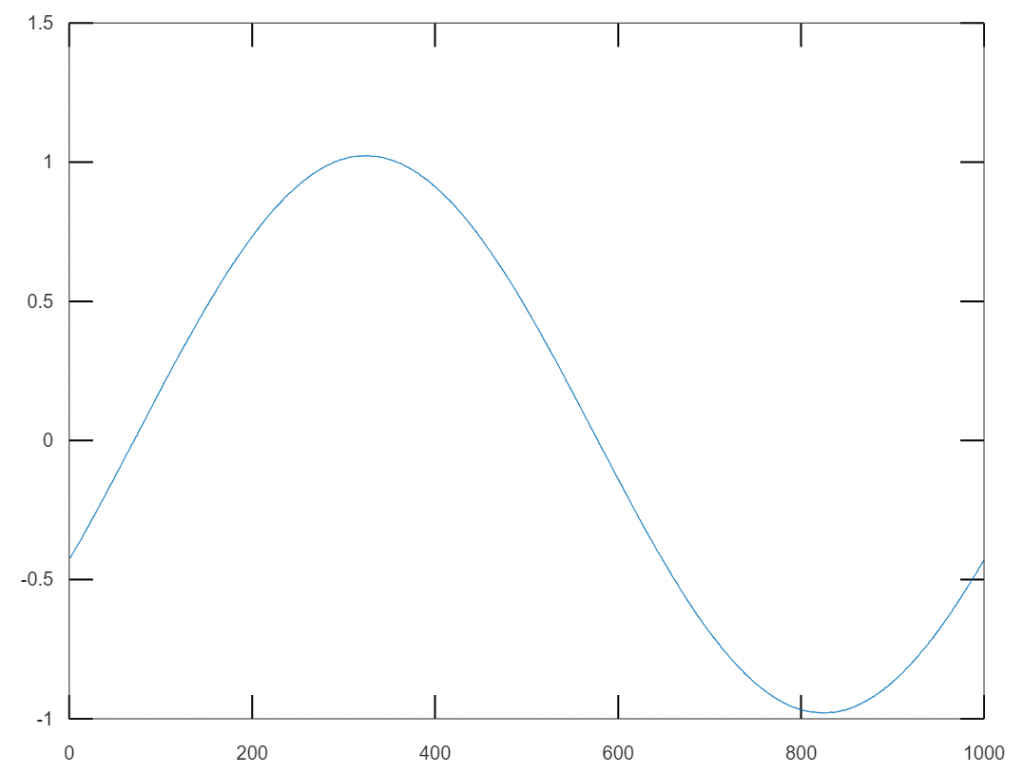
The acquired data is correct. I can see exactly one cycle of the 1Hz sinusoidal input waveform.
GUI
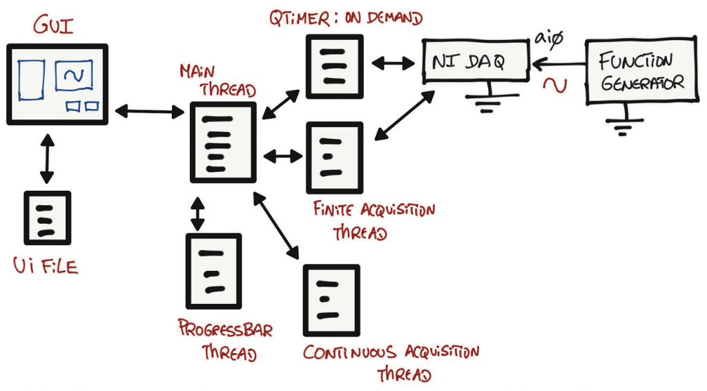
On this visualization method I replicated Figure 1 using PyQt6 and Qt Creator. If you are not familiar how to create GUIs, I recommend reading [Ref 3] first.
To run this example, you need the ni_daq_ai_single_continuous_gui.py and ni_max_Continuous.ui files available on the Python Files section.
Note: ni_max_Continuous.ui builds from ni_max_Finite.ui. If it is hard to follow the code for ni_daq_ai_single_continuous_gui.py, I would recommend understanding the code for the ni_daq_ai_single_finite_gui.py first and then understand the additional changes.
You can adjust the Rate and Samples to Read parameters according to your needs.
Code Diagrams
The goal with this section is to provide several different types of block diagrams that allow the understanding of the GUI code.
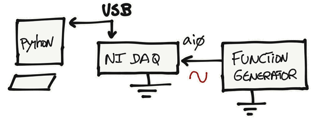
The first diagram is a generic block diagram on how the code, GUI, ui file and external hardware interact with each other in an conceptual way.
The second diagram was generated using code2flow and finds all function definitions in the code, and determines where those functions are called.
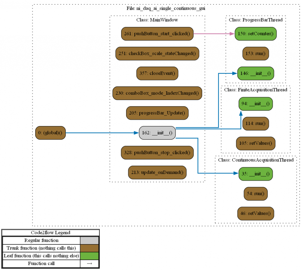
The above diagram provides a good estimate of the project's overall structure.
When not to use it...
If your goal is to capture and plot analog values without real time constraints, this mode might be a bit more complicated to set up that needed. Check on demand acquisition mode for acquiring/plotting data without real time constraints.
References
- [Ref 1] “Plotting with Matplotlib”, pythonguis Website [Article]
- [Ref 2] Pyqtgraph examples -> run command: python3 -m pyqtgraph.examples
- [Ref 3] “Simple Qt GUI”, EngrEDU Glue Article [Article]