Fourier vs Laplace
Another topic of great confusion while studying engineering: when to use Fourier Analysis or Laplace Transforms to tackle engineering problems. This article covers the differences and similarities and hopefully that helps clarifying which tool to use for your studies or projects.
Differential Equations
The main goal on using tools like Laplace transforms or Fourier analysis is to help understanding physical systems that are normally modeled by differential equations. Why differential equations? It is normally easier to measure or observe physical events that change over time. That change over time can be capture as a change rate, and change rates are represented in math language as derivatives. Differential equations are equations that relates one or more of those derivatives and they are present in a variety of different engineering topics.
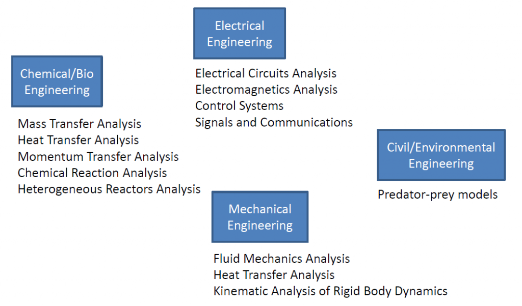
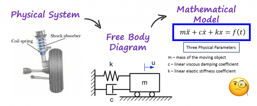
The process of studying a physical systems is normally divided into 2 main steps:
- the first step is the design of a model that abstracts the physical system to a certain degree. We try to capture in that model the physical elements that change over time.
- and the second step is the representation of that model by a mathematical model. We normally use equations to represent those physical elements that change over time.
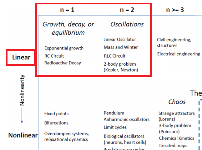
The world of differential equation is big, and when I say big, it is really big. In [Ref 2] you can find a table that attempts to organize and give a visualization of the different types of differential equations. n is related with the order of the differential equation.
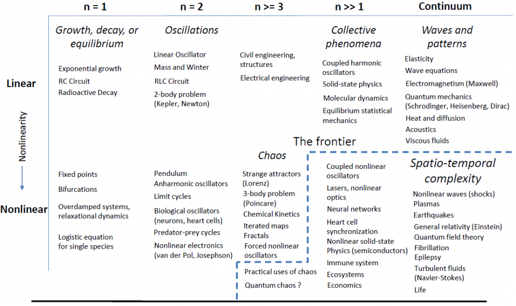
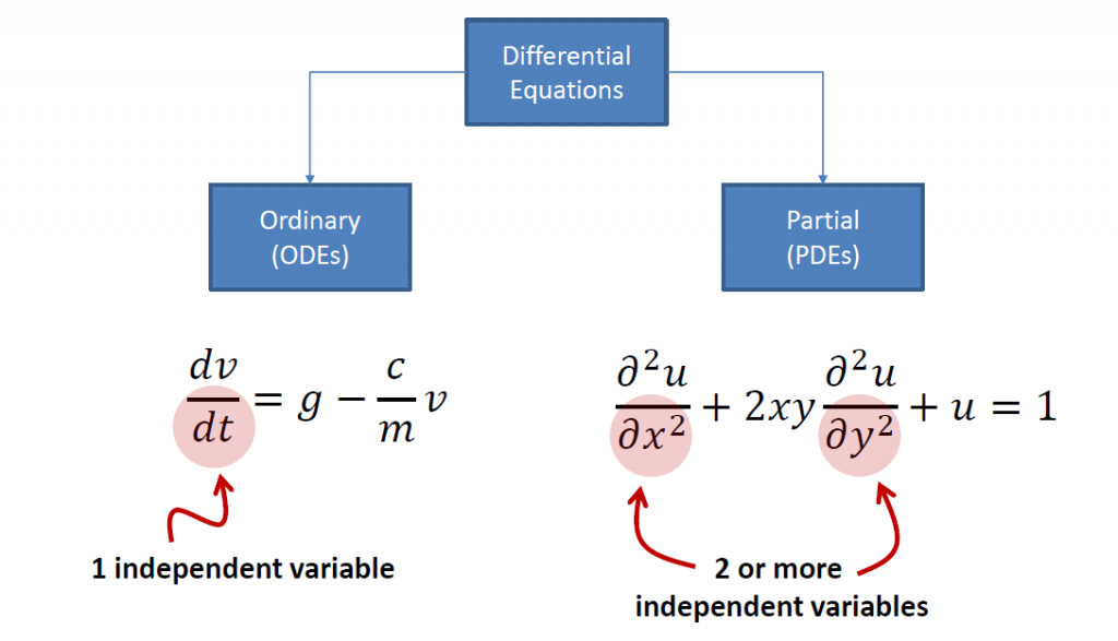
Differential equations are normally divided into 2 categories: Ordinary Differential Equations (ODEs) and Partial Differential Equations (PDEs).
Not all differential equations will have solutions, and there are tools that you can use to know if there is a solution or not (Uniqueness Theorems) for some of them. Just because we know that a solution to a certain differential equations exists does not mean that we will be able to find it. In this case, there are more tools (e.g., Numerical Methods) that we can use to get an idea of potential answers.
The way that we classify differential equations, determines which tool you should use to study them and get some answers.
This is a place where a lot of confusion starts rising. I believe the main reason why is because there are so many different types of differential equations that it is easy to get lost. For example, in this website you can find:
- 48 different types of 1st ODEs (Link)
- 50 different types of Linear 2nd ODEs (Link)
- 51 different types of Non Linear 2nd ODEs (Link)
- 16 different types of Linear Higher ODEs (Link)
- 12 different types of Non Linear Higher ODEs (Link)
For a good portion of the systems that you will be studying in the beginnings of an engineering degree, you will be facing with linear ODEs of first and second order that are Homogeneous or Non Homogeneous with constant coefficients (don't worry too much at this point what this mean, you will get exposed to these equations during a circuits or dynamics class). For these equations we can use with confidence Laplace and/or Fourier to study them. We will see later in this article in which situations we should use Laplace or Fourier to study this type of ODEs.
Real and Complex Exponential Signals
The previous section introduced the topic and the different types of differential equations. Before diving in into the connection between differential equations, Laplace and Fourier, I need to cover the difference between a real and a complex exponential function.
An exponential function can have different behaviors depending on which domain it is represented.
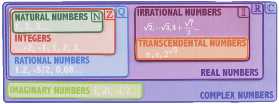
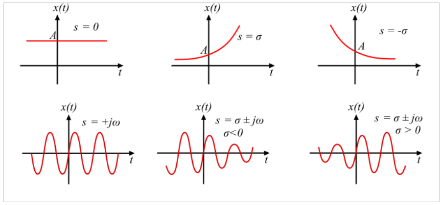
An exponential function, x(t) = Aeαt , with a real argument α, behaves in the following manner as we change the argument α.
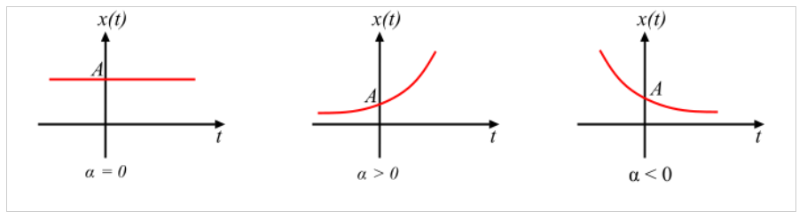
However, if that argument becomes a complex number, s = σ + jω, then we automatically switch to a different domain, the complex domain (
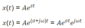
The complex exponential function has two interesting parts: a real exponential function (Aeσt) that shapes the magnitude of a complex exponential function (ejωt).
Since x(t) is a complex function, we have two options to be able to visualize what is going on. First option, we can visualize the function in the complex domain (
Visualization in the Complex Domain
We will start by visualizing x(t) by setting σ = 0, in the complex domain. That means that we will be working with x(t) = ejwt .
Since the majority of our graphing software works in the real domain (
I am not going to cover arithmetic operations in the complex plane on this article, but I will leave some animations for additions (Live Animation), subtractions (Line Animation), multiplication (Live Animation), and divisions (Live Animation), in case you need a quick review.
Note: The interesting part with the complex plane is the fact that you can treat complex points as vectors too.
When we want to plot a complex exponential function things start to get interesting. This is when Euler's formula comes into place. Euler's formula tells us that the real part of the complex number changes with the cosine function while the imaginary part changes with the sine function. With this we can make ejwt = ejθ
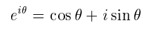
If we plot this exponential function in the complex plane, we get a complex point (black point below) that rotates as we change the argument (θ). (Live Animation)
Since the complex plane is "borrowing" the axis of the real domain (
Visualization in the Real Domain
To visualize x(t) = ejwt in the real domain (
Remember that the complex plane is "borrowing" the axis of the real domain (
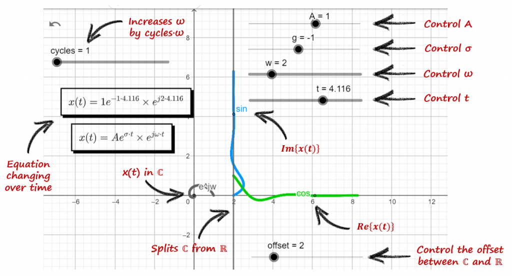
Let's proceed with the plot of x(t) = Aeσt ejwt in the complex and real domains and see what type of plots we get. You can use the live animation on this link (Link) to confirm the results, and play around with different settings and see what you get.
Animation Guide
Remember that the complex plane is "borrowing" the axis from the real domain. We can plot both graphs at the same time, but they are representing different information. I am using a gray line on the x axis to divide
Re\left\{ x(t) \right\}
=
Re\left\{ Ae^{\sigma t} . e^{j\omega t} \right\}
=
Re\left\{ Ae^{\sigma t} . \left[ cos(\omega t) + jsin(\omega t) \right] \right\}  \\
\color{red} Re\left\{ x(t) \right\} \color{black} = Ae^{\sigma t} . cos(\omega t)
Im\left\{ x(t) \right\}
=
Im\left\{ Ae^{\sigma t} . e^{j\omega t} \right\}
=
Im\left\{ Ae^{\sigma t} . \left[ cos(\omega t) + jsin(\omega t) \right] \right\}\\
\color{red} Im\left\{ x(t) \right\} \color{black} = Ae^{\sigma t} . sin(\omega t)s = 0
For s = 0 → σ + jω = 0 + j0, both exponential functions are equal to 1 and x(t) = A.
x(t) = Ae^{\sigma t}.e^{j\omega t}|_{s=0} = Ae^{0} . e^{0}=A
In the complex domain, there is no rotation, and the value of A is a point along the real axis. In the real domain, the green line is equal to A and the blue line is equal to 0.
s = σ
With σ > 0 and ω = 0 → σ + jω = +σ + j0, x(t) has the same response has a real exponential function with a positive exponent.
x(t) = Ae^{\sigma t}.e^{j\omega t}|_{s=\sigma} = Ae^{\sigma t} . e^{0}=Ae^{\sigma t}
In the complex domain we have the point moving along the real axis growing to +∞. In the real domain the green line moves according to an exponential function with a positive exponent, and the blue line is zero.
s = -σ
With σ < 0 and ω = 0 → σ + jω = -σ + j0, x(t) has the same response has a real exponential function with a negative exponent. The complex exponential function (ejωt) is still equal to 1.
x(t) = Ae^{\sigma t}.e^{j\omega t}|_{s=-\sigma} = Ae^{-\sigma t} . e^{0}=Ae^{-\sigma t}
In the complex domain we have the point moving along the real axis decaying to zero. In the real domain the green line moves according to a negative exponential function with a negative exponent, and the blue line is zero.
s = jω
With σ = 0 and varying ω → σ + jω = 0 + jω, we get an oscillatory response. The same result from when we plot the complex exponential function before.
x(t) = Ae^{\sigma t}.e^{j\omega t}|_{s=jw} = Ae^{0} . e^{jwt}=Ae^{jwt}
s = - σ ± jω
With σ < 0 and varying ω → σ + jω = -σ ± jω, we observe some interesting stuff. Notice on how the Re{x(t)} and the Im{x(t)} have similar responses, shiftet by 90 degrees.
x(t) = Ae^{-\sigma t}.e^{\pm j\omega t}
Turning off the Im{x(t)}, and keeping just the Re{x(t)}, we observe that the real exponential function (Aeσt) shapes the complex exponential function (ejωt). With σ < 0 the response of Aeσt tends to zero, shaping the oscillatory motion from ejωt to zero.
In the complex domain, the point moves to zero as a seashell shape :).
s = σ ± jω
With σ > 0 and varying ω → σ + jω = +σ ± jω, we observe that the real exponential function (Aeσt) shapes the complex exponential function (ejωt). With σ > 0 the response of Aeσt tends to +∞, shaping the oscillatory motion from ejωt to +∞. It enters in what it is called an unstable state.
x(t) = Ae^{\sigma t}.e^{\pm j\omega t}
In summary we get the following plots for Re{x(t)} in time (real domain).
Fourier Analysis
The goal with this section is to complement any other resources about Fourier analysis. Fourier analysis is an extensive topic and it would be overwhelming to cover all that information here. I am selecting the essential knowledge that can help with the understanding of the main topic.
There are different types of Fourier functions (you can read the "Types of Fourier" section under the Fourier Analysis article), but for this article we will focus on the Fourier transform applied to continuous signals.
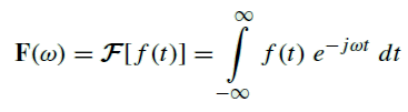
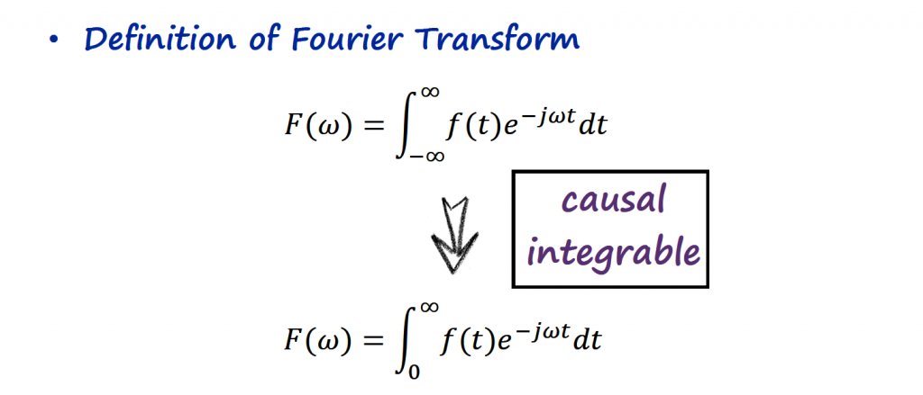
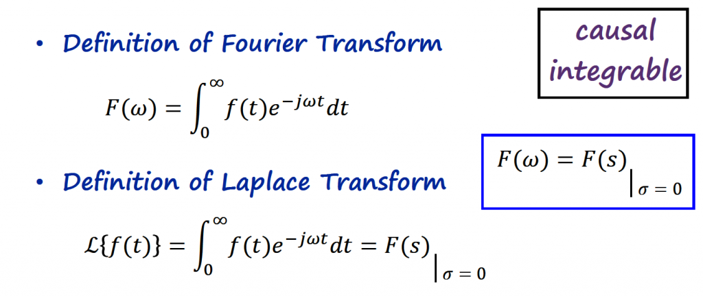
The formal definition of the Fourier transform is the following:
If you would like to know more on how to get to this equation you can read the "Fourier Transform" section under the Fourier Analysis article.
What this equation is telling us, and I know it is hard to see it in this form, is that we can describe a function f(t) as a summation of infinity harmonically related complex sinusoids.
- The complex sinusoids are being represented by the Euler's formula, e-jwt
- The summation is being represented by the integral → ∫
- The infinity is being represented by the limits of integration ±∞
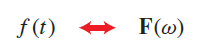
Occasionally, we also may use the symbolic form
For now we will leave the Fourier transform here. Remember this equation, because it will be useful later.
Laplace Analysis
The goal with this section is to complement any other resource about Laplace analysis. Laplace analysis is an extensive topic and it would be overwhelming to cover all that information here. I am selecting the essential knowledge that can help with the understanding of the main topic.
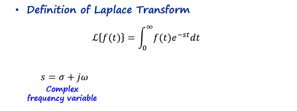
The Laplace transform is a mathematical tool that it is used to study physical systems that are modeled by Linear ODEs in specific the Homogeneous and Non Homogeneous type with constant coefficients. There are two flavors for writing the general equation, the unilateral and bilateral Laplace transform.
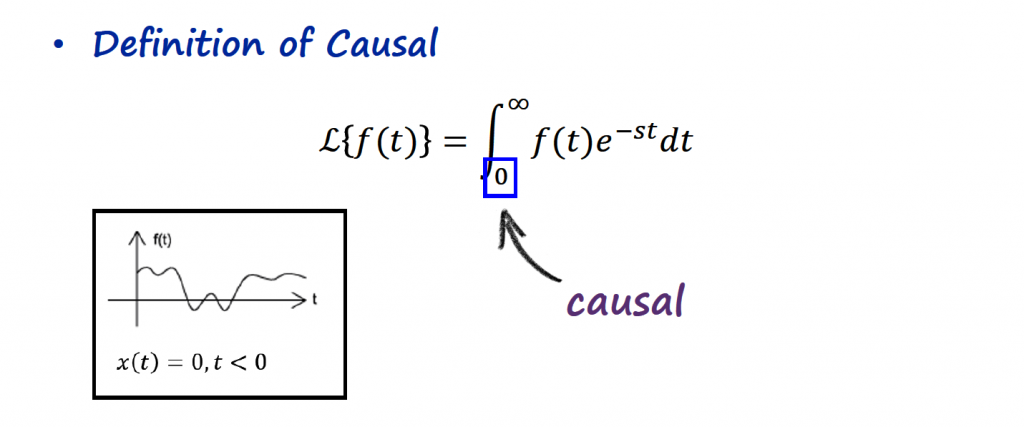
The unilateral Laplace transform is defined by
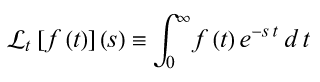
where f(t) is defined for t ≥ 0. The unilateral Laplace is almost always what is meant by "the" Laplace transform, although a bilateral Laplace transform is defined as
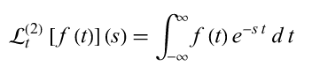
Since we are dealing with physical systems for engineering topics, the concept of negative time doesn't really apply and we use the unilateral Laplace transform.
I hope by now you can recognize the e-st portion of the equation. We have a complex exponential function involved in the Laplace transform, that can be expanded to e-(σ+ω)t which in turn becomes e-σt . e-jωt
That tells that the Laplace relates by integration a bunch of exponentials and sinusoidal waveforms with the function f(t). Since the constant of integration is time (t), s (complex number) is considered a constant and we perform the integration with respect to time.
Laplace Integration
To help understanding the integral, I am going to select an f(t) that it is easy to solve. The input function will be an exponential function → f(t) = e-αt
F(s) = \int_{0 }^{+\infty} f(t)e^{-st}dt
=
\int_{0 }^{+\infty} e^{-\alpha t}e^{-st}dt
F(s) = \int_{0 }^{+\infty} e^{-\left( \alpha + s \right)t}dt
=
\left[ -\frac{e^{-\left( \alpha + s \right)t}}{(\alpha+s))} \right]_{0}^{+\infty}
=
e^{-\infty} - \left[ -\frac{e^{0}}{\alpha+a} \right]F(s) = \frac{1}{s+\alpha}We get an equation in the Laplace domain, where the input (s) is a complex number (a+jb) and outputs another complex number (a+jb).
F(a+jb) = \frac{1}{a + jb+\alpha}To plot this equation in the complex domain, remember that we are "borrowing" the real domain (
F(a+jb) = \frac{a+\alpha}{\left(a+\alpha \right)^2+b^2}+j\frac{-b}{\left(a+\alpha \right)^2+b^2}Now we are ready to start plotting things around, and let's start by visualizing the output in the complex domain.
Output Plot
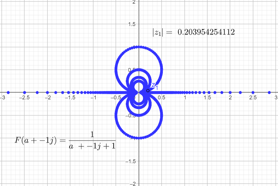
You can use this link to run the animation below by yourself. It would be interesting to plug other functions and see what you get. If you change the function, don't forget to adjust the z1 point coordinates accordingly.
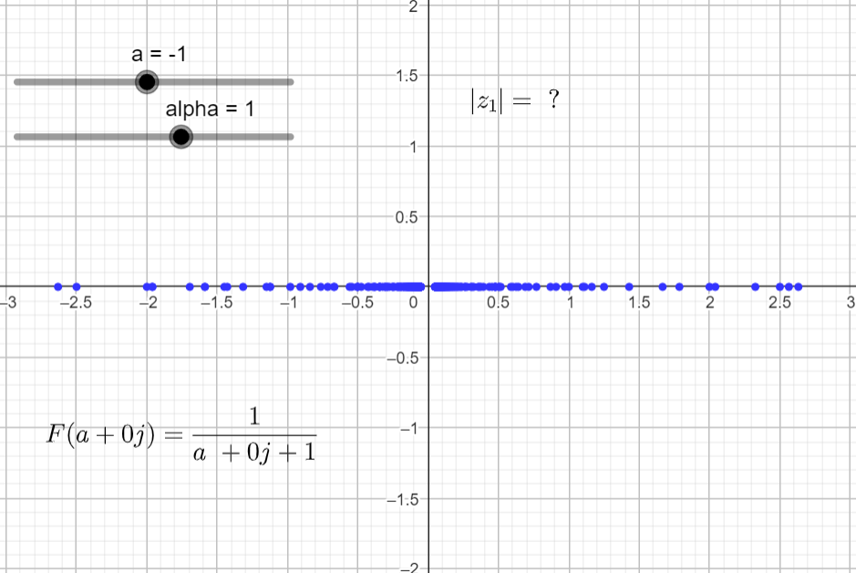
I am going to set α=1, b=0 and vary a:
F(a+j0) = \frac{1}{s+\alpha} = \frac{1}{a + j0+ 1}
Increase b and vary a:
Decrease b and vary a:
Final rendering with more points.
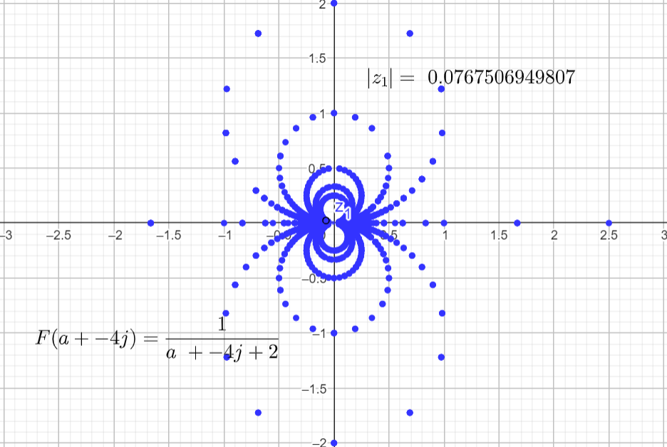
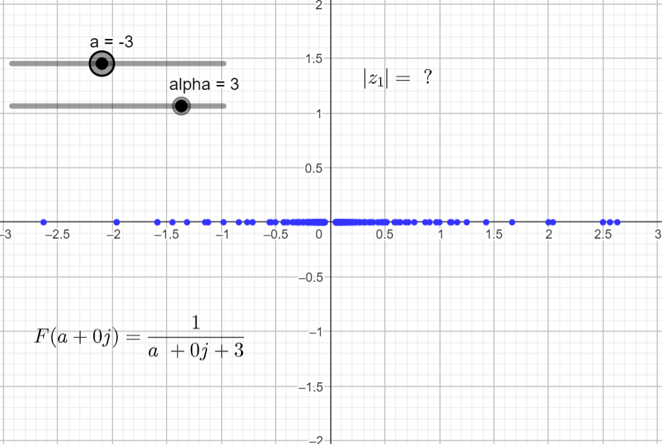
If we set α=2, and repeat the same steps we get the final output plot.
If we set α=5, and repeat the same steps we get the final output plot.
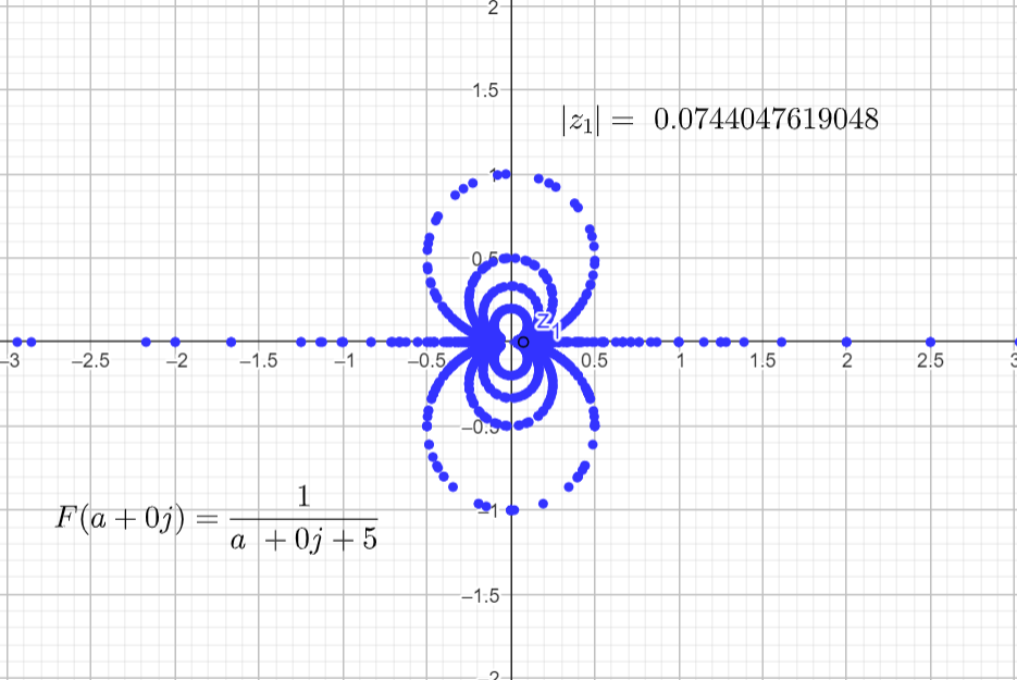
It seems that the plots in the complex domain are all the same for different α's. But there is a small nuance that it is hard to spot while rendering this function. For ω = 0 and a = -α the function is undefined because:
F(-1+j0) = \frac{1}{s+\alpha} = \frac{1}{-1 + j0+ 1}=\frac{1}{0}To catch this detail, since I am in the complex domain and I am plotting complex numbers with cartesian coordinates, I can convert this number to polar coordinates and have a look at the magnitude of the complex number.
z_{1}=\left|s\right|\angle \phi \\
\left|s\right|=\sqrt{a^2+b^2} \\
\phi=tan^{-1}\left( \frac{b}{a} \right)
The pictures below show the magnitude of F(s) = |z1| for different α's and when a=-α.
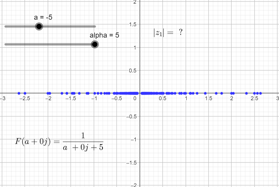
It will be interesting to plot this information in a different way, that would allow to capture this undefined value.
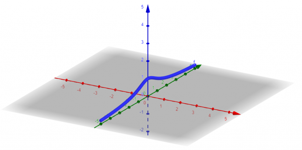
Input Plot
From the output plot section we observed that it would be interesting somehow to plot the magnitude of F(s). Since we have a complex number (a+jb) plus a magnitude, we need to do a 3D plot, where the x axis = a, the y axis = b, and the z axis = |F(s)|.
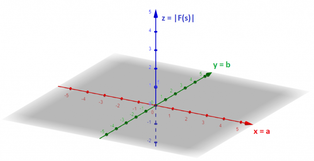
You can use this link to reproduce this results and play around with different functions if you want.
Recall the function that we are using as an example:
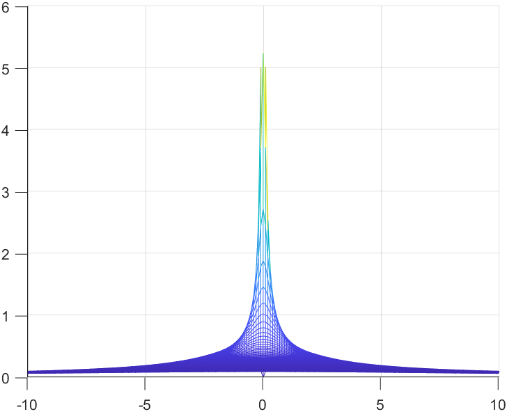
F(a+jb) = \frac{1}{s+\alpha} = \frac{1}{a + jb+ \alpha}I will set α=1, and for every blue line in the plot below I am setting a value for a and sweep b input. Then I move a to a new value and sweep b input again.
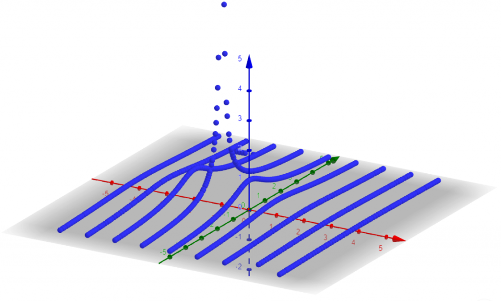
Then I do the opposite, I set a value for b and sweep a input.
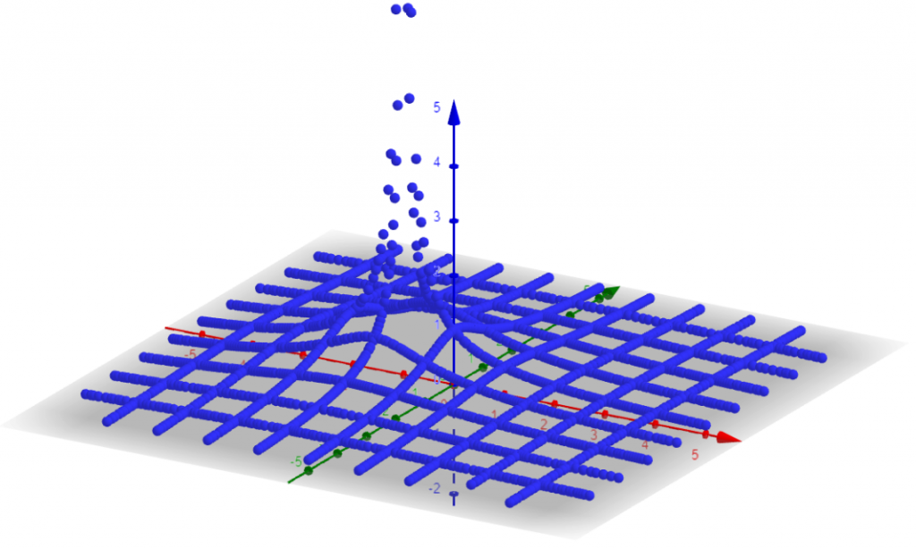
We are getting somewhere. The point where a = -α goes to infinity 🙂
I admit that rendering images like this is cool, but I need to find a faster way to render this information.
I am going to use MatLab to help me from this point on. If you don't have a license for MatLab, you can use an equivalent free software called Octave. The commands will be the same.
First I prepare the grid to plot complex numbers. I also set s to be a complex number and use X as the real part and Y as the imaginary part. Z is filled with zeros for now.
[X,Y] = meshgrid(-10:0.1:10);
Z = zeros(201, 201);
s = X + 1i*Y;
mesh(X,Y,Z)
Plotting this, we have an empty meshgrid.
Now we are in good shape to add the code to plot the input values vs magnitude of our function F(s). All we need to do is to set Z equal to the magnitude of F(s).
F(s) = \frac{1}{s+\alpha}a = 1;
Z = abs(1./(s+a));
mesh(X,Y,Z);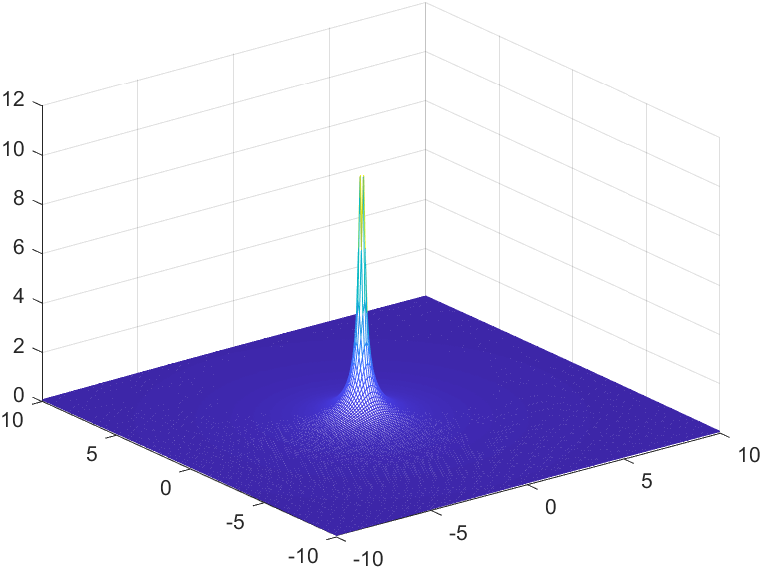
Voila, we get the same result, and we can plot other functions way faster.
Moving the Input Plot Around
Let's rotate the meshgrid around and get familiar with some shapes and information. The figures below are related with the following Laplace function:
F(s) = \frac{1}{s+\alpha}|_{\alpha=1}=\frac{1}{s+1}Top View (XY View)

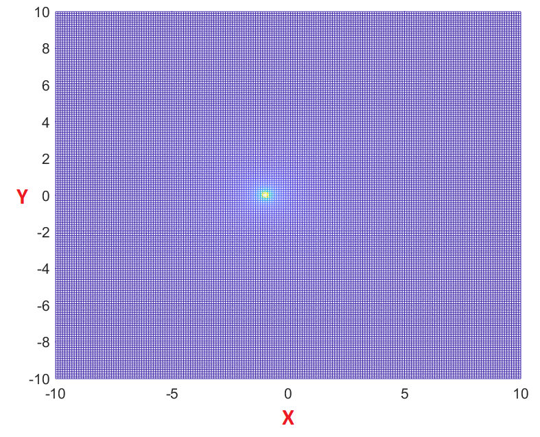
This is an interesting view where I can see the a and b coordinates from the output plot where the value of F(s) was undefined.
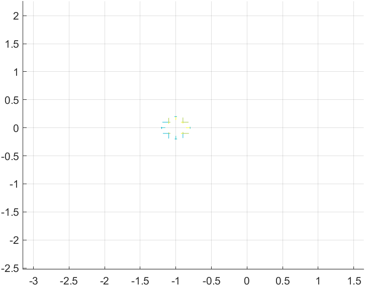
Zoom in and you can validate that a+jb = -1 +j0
XZ View
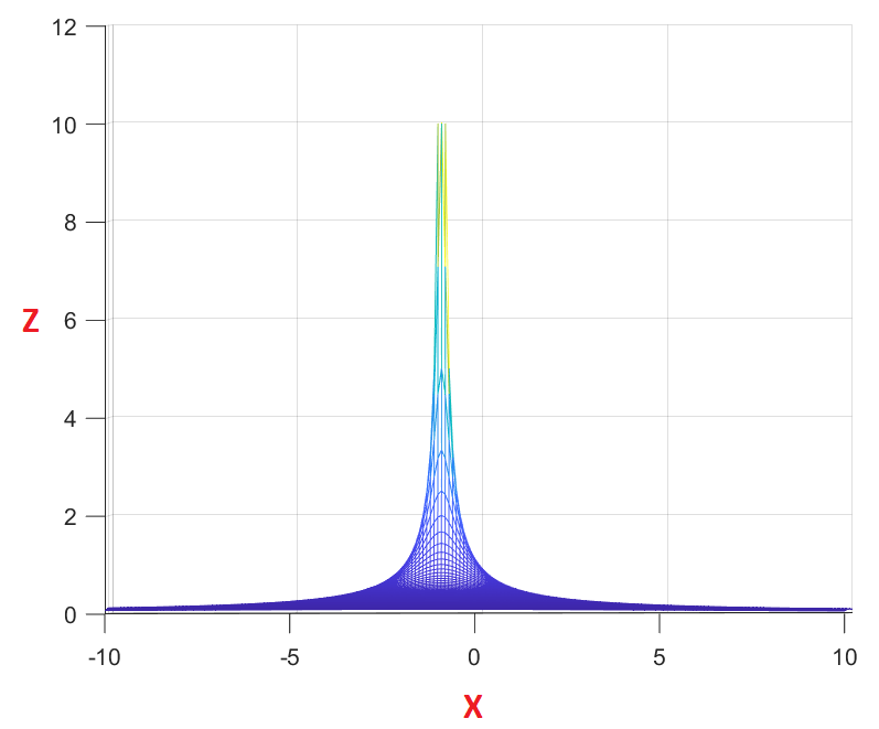
From this view we can see that we have an undefined point with x = -1.
YZ View

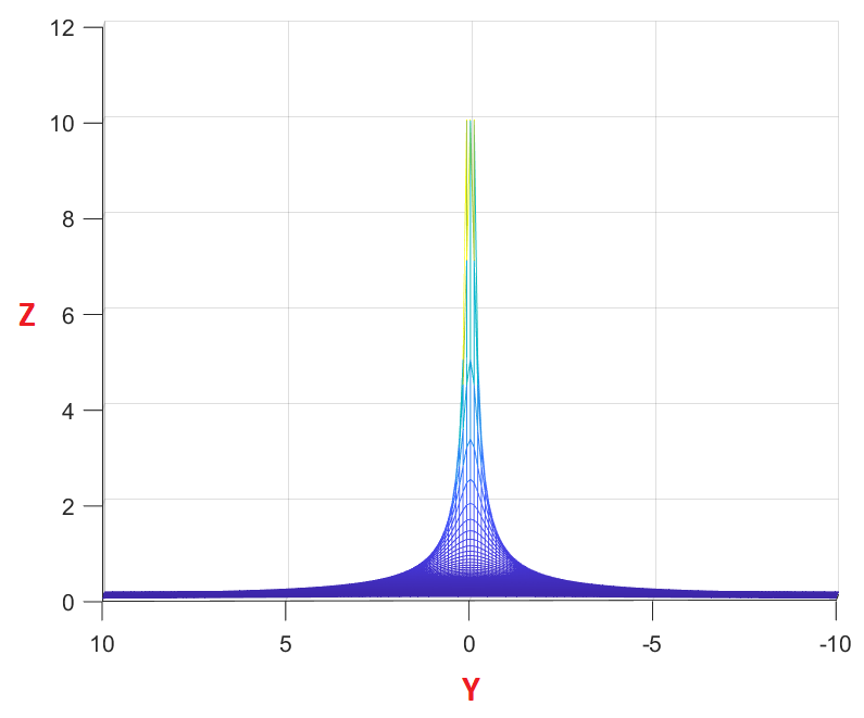
From this view we can see that the undefined point has a value of y = 0.
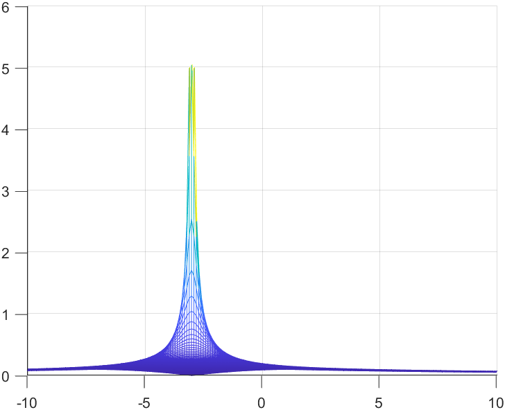
Let's repeat this process but for a different input function → f(t) = cos(ωt). The steps are going to be the same as before, but I will provide only the results for this time.
F(s) = \int_{0 }^{+\infty} f(t)e^{-st}dt
=
\int_{0 }^{+\infty} cos\left(\omega t\right)e^{-st}dtF(s) = \frac{s}{s^2+\omega^{2}}F(a+jb) = \frac{s}{\left( a+jb \right)^2+\omega^{2}}Results below are for ω = 1
Results
Top View
Zoom in and you can see that we have two undefined values this time, ±j1. Notice that the value of b sits at plus or minus the the initial value of ω = 1.
XZ View
From this view we can see that the undefined points have a value of x = 0.
YZ View
From this view we can see that the undefined points have values at y = ±1 respectively.
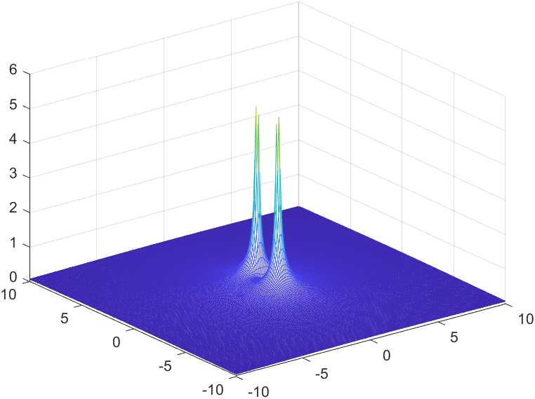
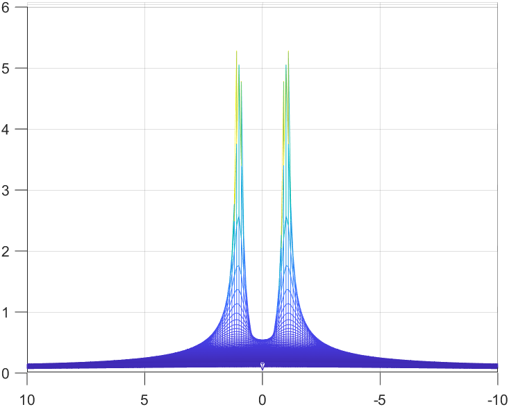
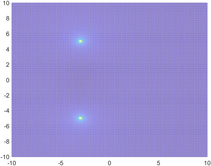
Let's do one more but now let's combine an exponential with a sinusoidal function → f(t) = e-αt . cos(ωt)
F(s) = \int_{0 }^{+\infty} f(t)e^{-st}dt
=
\int_{0 }^{+\infty} e^{-\alpha t}cos\left(\omega t\right)e^{-st}dtF(s) = \frac{s+\alpha}{\left( s+\alpha \right)^2+\omega^{2}}F(a+jb) = \frac{(a+jb)+\alpha}{\left( (a+jb)+\alpha \right)^2+\omega^{2}}Results below are for ω = 5, α =3
Results
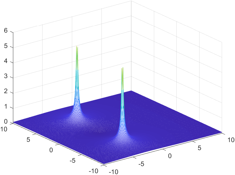
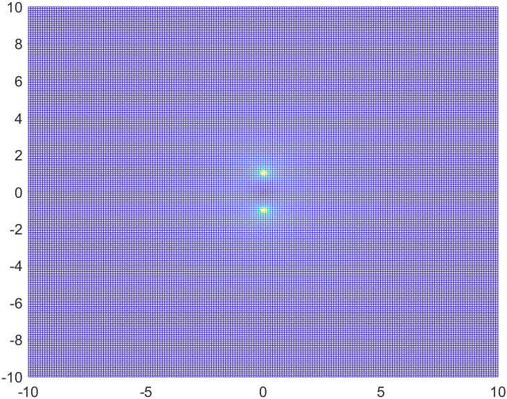
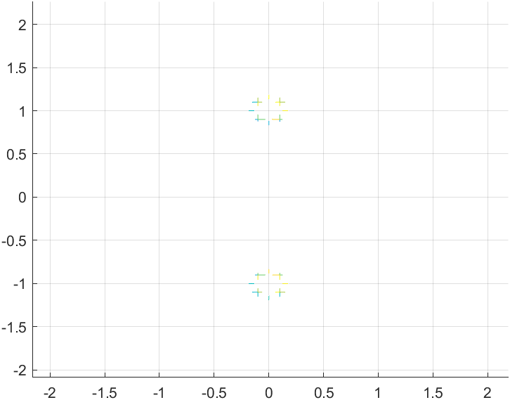
Top View
XZ View
From this view we can see that the undefined points have a value of x = 3.
YZ View
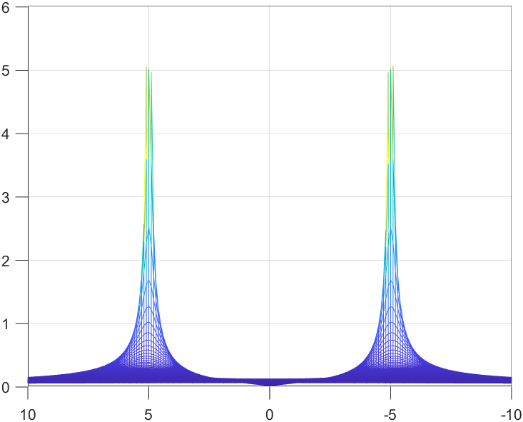
From this view we can see that the undefined point have a value of y = ±5.
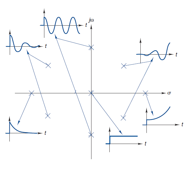
If we proceed with the same test for different combinations of exponential functions and cosine functions we can create the plot below that relates f(t) with the XY axis from the input plot of the Laplace transform. Remember that the XY view shows the undefined points from the Laplace transform (F(s)).
Fourier Transform Connection
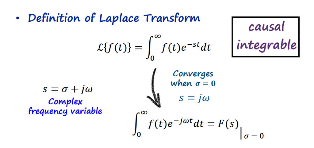
If we set σ = 0 on the Laplace transform, we get the following:
F(0+j\omega)
=
\int_{-\infty}^{+\infty}f(t)e^{0 t}e^{-j\omega t}dt
=
\int_{-\infty}^{+\infty}f(t)e^{-j\omega t}dtYou get the same expression as the Fourier transform.
Since we are dealing with physical systems in engineering (t > 0), we can focus our attention to the unilateral version of this equation.
F(0+j\omega) = F(\omega)
=
\int_{0}^{+\infty}f(t)e^{-j\omega t}dtThat tells us that the Fourier transform is a present in the Laplace transform, and it will be the plot in the complex domain where σ = 0.
Let's go back to the simple example of f(t) = e-αt and repeat some plots that we did on the previous section to understand this connection visually.
F(s) = \int_{0}^{+\infty}f(t)e^{-j\omega t}dt
= \int_{0}^{+\infty}e^{-(\alpha + j\omega) t}dt F(0 + j\omega) = \frac{1}{j\omega+\alpha} Setting α = 1, and plotting the magnitude of F(s) vs the input values (a + jb → 0 + jb), we get the following:
Superimposing this answer with the previous Laplace 3D plot for the same F(s), we confirm that the Fourier transform is present in the Laplace.
Using MatLab we can start by plotting the Laplace of the desired function as we did before.
[X,Y] = meshgrid(-10:0.1:10);
Z = zeros(201, 201);
s = X + 1i*Y;
mesh(X,Y,Z)
a = 1;
Z = abs(1./(s+a));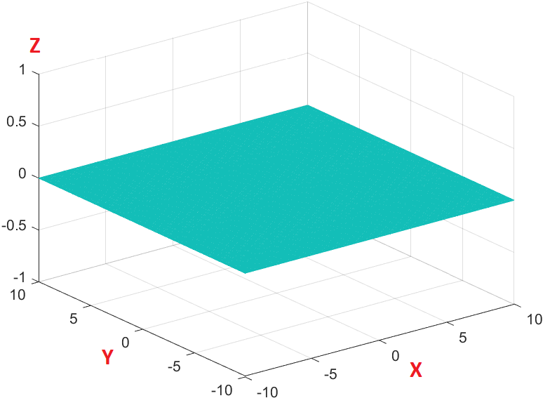
mesh(X,Y,Z);And then add the plane that intersects x = σ = 0. The command hold on and hold off is used to make sure that what is in between those instructions gets superimposed to the previous mesh.
hold on

[Y,Z] = meshgrid(-10:0.1:10);
X = zeros(201, 201);
mesh(X,Y,Z);

hold off
The intersection is the Fourier transform result.
s-Plane
Before continuing with this section, make sure that you digested the information from the previous sections. The contents from this section are based on previous results that we have been plotting.
Once again I am going to use examples to explain the concept of s-Plane (or Argand diagrams), transfer functions, and region of convergence.
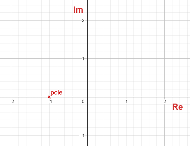
F(s) = \frac{1}{s+\alpha} |_{\alpha = 1}=\frac{1}{s+1}The XY (Top View) plot that we got in the "Laplace Analysis" section, has information about the values of s that makes the function undefined. Moreover we can see that in this case, this happen when s = -1.
Notice that s = -1 is the root of the polynomial that is the denominator of F(s). We call the roots of this polynomial poles, and if we have a polynomial as numerator, we will call the roots, zeros. I will cover a couple more examples below.
We also call F(s) a transfer function. In the Laplace domain, transfer functions are always polynomials. That is one of the strengths of Laplace transform, we can convert differential equations in time to s-domain, and we are dealing with polynomials that are easier to manipulate and find solutions for.
We can plot these poles and zeros directly in the XY plot. This XY plot is called s-Plane or Argand diagrams. Poles are marked with an "x", and zeros are marked with a "o".
s-Plane Examples
Let's see more examples, and calculate the roots of the functions, plot the poles and zeros in the s-Plane and compare the results with the XY plot done with MatLab.
Example 1
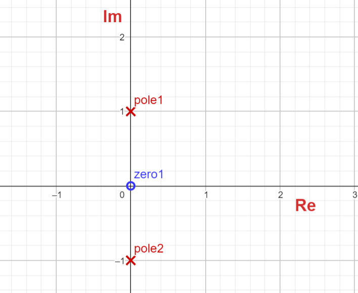
F(s) = \frac{s}{s^2+\omega^{2}}Roots of the numerator (zero): s = 0
Roots of the denominator (poles):
s^2+\omega^2=0 \to quadratic \ equation\\
as^2 + bs + c = 0\to find  \ solution
s = \frac{-b\pm \sqrt{b^2 - 4ac}}{2a} s = \frac{0\pm \sqrt{0-4w^2}}{2}=\pm jwSetting ω = 1, we get the following s-Plane plot (manual):
XY Plot with MatLab.
[X,Y] = meshgrid(-10:0.1:10);
Z = zeros(201, 201);
s = X + 1i*Y;
mesh(X,Y,Z)

w = 1;
Z = abs(s./(s.^2+w.^2));
mesh(X,Y,Z);
At this point we know that poles correspond to values where F(s) is undefined, or F(s) = 1/0. On the other hand, zeros are related with values where F(s) = 0.
In this case we have one zero at (0,0). We confirm the same values that we plotted by hand.
We can use MatLab to find the poles and zeros, and plot them directly on the s-Plane.
numerator = [1 0];
denominator = [1, 0, 1];
F = tf(numerator, denominator);

%Plot Poles and Zeros
pzmap(F)
grid, axis([-2 0 -1 1])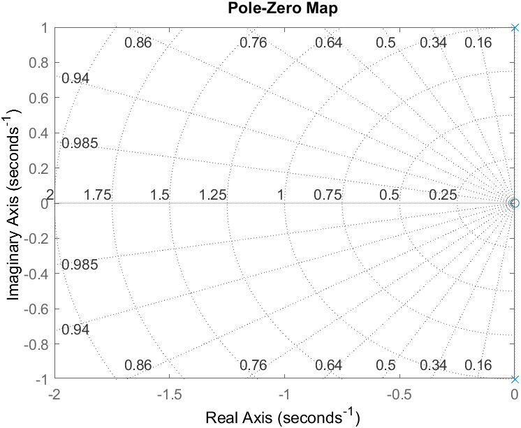
Example 2
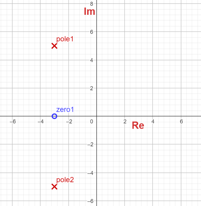
F(s) = \frac{s + \alpha}{(s + \alpha)^2+\omega^{2}}Zeros: s = -α
Poles:
s^2+2\alpha s+(\alpha^2+w^2)=0
s = \frac{-2\alpha \pm \sqrt{(2\alpha)^2-4(\alpha^2+w^2)}}{2}=-\alpha + jwSetting α = 3, and ω = 5, we get the following s-Plane plot (manual):
XY Plot with MatLab.
[X,Y] = meshgrid(-10:0.1:10);
Z = zeros(201, 201);
s = X + 1i*Y;
mesh(X,Y,Z)

a = 3;
w = 5;
Z = abs((s+a)./((s+a).^2+w.^2))
mesh(X,Y,Z);
Plot poles and zeros with MatLab.
numerator = [1 3];
denominator = [1, 6, 34];
F = tf(numerator, denominator);

%Plot Poles and Zeros
pzmap(F)
grid, axis([-4 0 -6 6])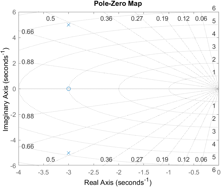
Normally, in signal processing, control, circuits (with memory elements), dynamics classes you learn how to check for the stability of signals and systems.
Stability Information
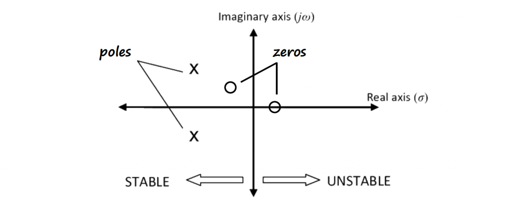
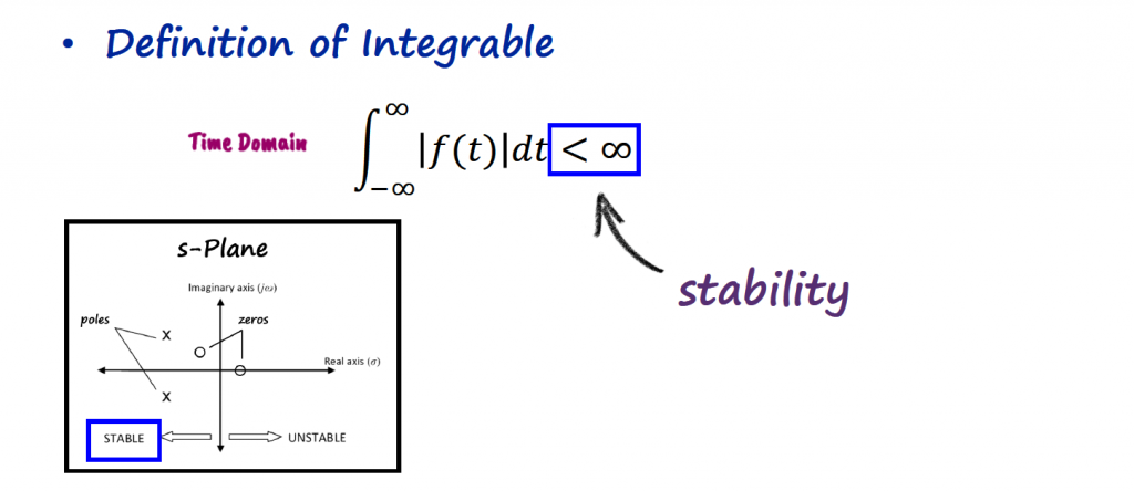
Another information that we can get from these s-Plane plots, is if your transfer function has a stable or unstable behavior based on where the poles are placed.
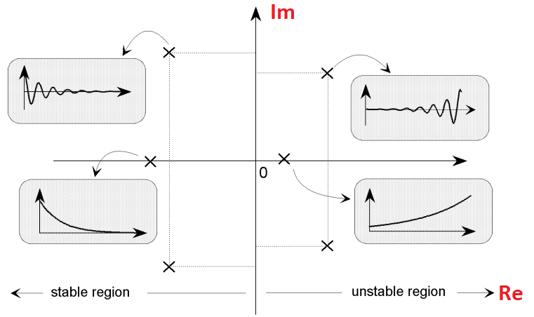
If the poles are in the left side of the s-Plane, your function is stable. That makes sense since all the time domain input functions on that side of the plane are related with exponential functions with negative exponent that forces the response to decay to zero. If you have at least one pole on the right side of the s-Plane, your function is unstable, since the response is increasing to +∞.
A system can be marginally stable when at least one pole of its transfer function lies on the jω axis of the s-Plane.
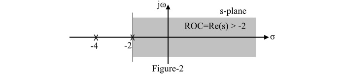
Region of Convergence
The Region of Convergence (ROC) is defined as the set of points in s-Plane for which the Laplace transform of a function f(t) converges. In other words, the range of Re{s} or F(σ), for which the function F(s) converges.
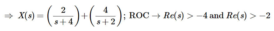
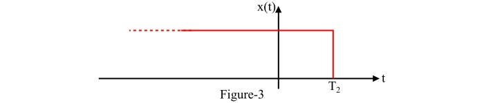
ROC of Right-Sided Signals
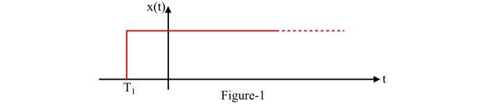
For a right-sided signal x(t), the ROC of the Laplace transform X(s) is the following:
- Find the poles of X(s)
- The ROC is the region that extends rightward from the pole with the largest real-part (but not at infinity).
- No pole should exist inside the ROC region.
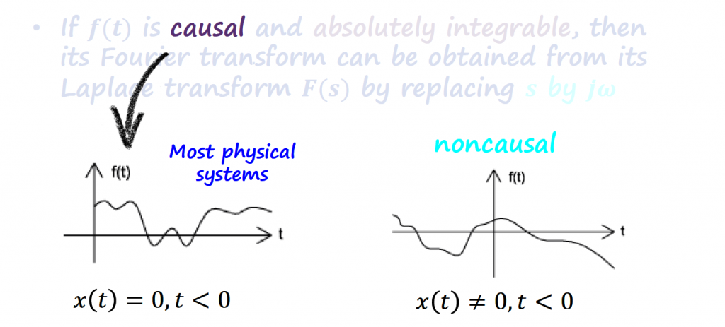
A causal signal is an example of a right-sided signal.
Example:
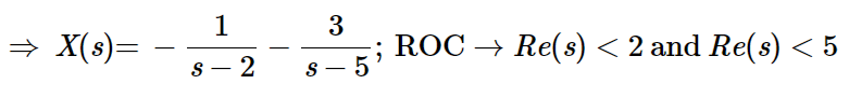
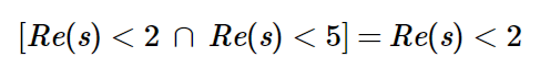
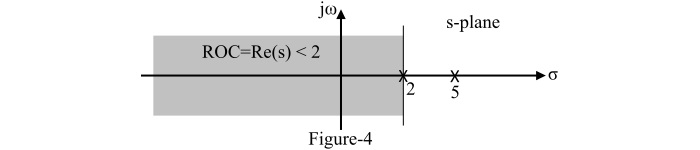
ROC of Left-Sided Signals
For a left-sided signal x(t), the ROC of the Laplace transform X(s) is the following:
- Find the poles of X(s)
- The ROC is the region that extends leftward from the pole with the smallest real-part (but not at negative infinity).
- No pole should exist inside the ROC region.
A anti-causal signal is an example of a left-sided signal.
Example:
Fourier vs Laplace
When to use Fourier or Laplace transform?
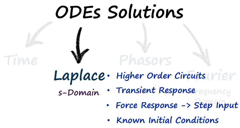
Laplace transform is useful when the differential equations have order higher or equal to 2, and you want to study the transient, and forced response to a step input. One thing to have in mind with Laplace is that it requires to know the initial conditions.
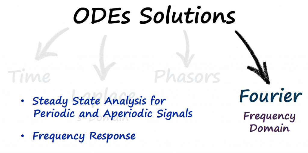
On the other hand, if you are interested in studying the frequency response of a steady state of a periodic or aperiodic signal, then Fourier analysis is the way to go. You don't need to know any initial conditions.
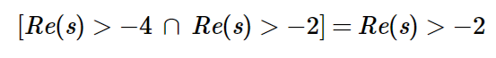
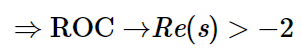
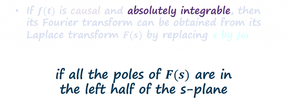
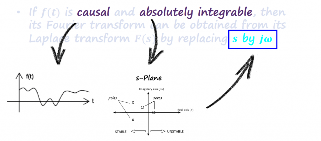
It is also common to find times the use of both analysis at the same time by substituting s = jω. In order to do this, we need to check some conditions:
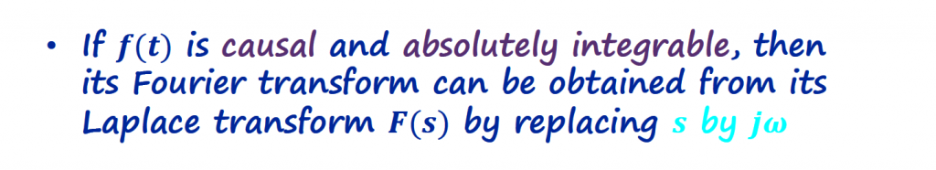
We can check these conditions in visual or mathematical way.
Visual Explanation
Mathematical Explanation
References
- [Ref 1] “Intuitive Guide for Fourier Analysis and Spectral Estimation”, Charan Langton and Victor Levin [Book]
- [Ref 2] “Nonlinear Dynamics and Chaos - With Applications to Physics, Biology, Chemistry, and Engineering”, Steven H. Strogatz [Book]
YouTube Videos
- [Ref 2] “The intuition behind Fourier and Laplace transforms I was never taught in school”, ZachStar [Video]
- [Ref 3] “What does the Laplace Transform really tell us? A visual explanation (plus applications)”, ZachStar [Video]
- [Ref 5] “Laplace Transform Explained and Visualized Intuitively”, Physics Videos [Video]
Other Resources
- [Ref 4] “The World of Mathematical Equations”, EqWorld [Website]