Fourier Analysis
Fourier analysis is the study of the way general functions may be represented or approximated by sums of simpler trigonometric functions. There are so many flavors under this Fourier analysis that it becomes confusing to understand which one to use. The goal with this article is to bring clarity to the different types of Fourier analysis and hopefully help with the understanding when to use the right form for your needs.
Types of Fourier
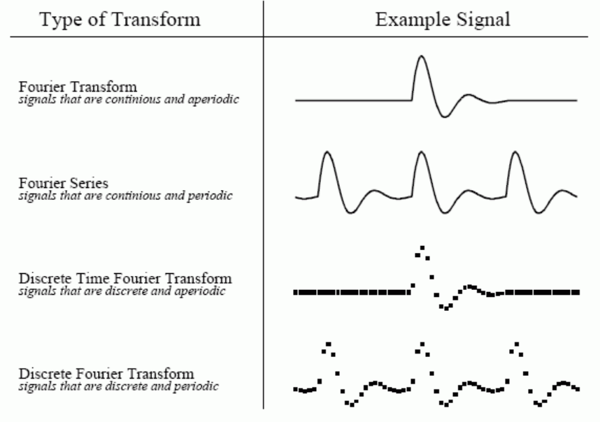
A signal can be either continuous or discrete, and it can be either periodic or aperiodic. The combination of these two features generates the four categories, described and illustrated below.
Continuous Signals
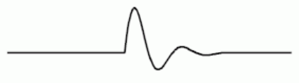
Fourier Transform
Aperiodic-continuous signals include, for example, decaying exponentials (or transients), the Gaussian curve, and noise. These signals extend to both positive and negative infinity without repeating in a periodic pattern. The Fourier analysis for this type of signal is simply called the Fourier Transform.
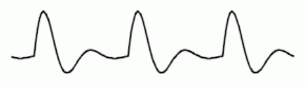
Fourier Series
Probably the most famous form, named after Joseph Fourier, who showed that representing a function as a sum of trigonometric functions greatly simplified the study of heat transfer. Here the examples include: sine waves, square waves, and any waveform that repeats itself in a regular pattern from negative to positive infinity. This version is called the Fourier Series.
Discrete Signals
DTFT
These signals are only defined at discrete points between positive and negative infinity, and do not repeat themselves in a periodic fashion. This type of Fourier analysis is called the Discrete Time Fourier Transform (DTFT).

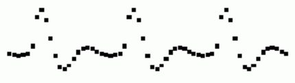
DFT
These are discrete signals that repeat themselves in a periodic fashion from negative to positive infinity. This class of Fourier analysis is sometimes called the Discrete Fourier Series, but is most often called the Discrete Fourier Transform.
When you struggle with theoretical issues, grapple with homework problems, and ponder mathematical mysteries, you may find yourself using the first three members of the Fourier analysis family. When you sit down to your computer, you will only use the DFT.
Fourier Series
A good portion of engineering topics (e.g., analog circuits, power, electromagnetics, signals and systems, engineering mathematics, digital communications), rely on Fourier series as a tool to study the problems that are present in those domains. That is the motivation behind starting with Fourier series on this article.
Fourier series deals with periodic signals that can be written as an infinite sum of harmonically related sinusoids.
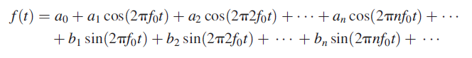
The confusion can start right here, there are 3 common forms to represent this infinite sum of sinusoids: trigonometric, cosine and exponential form.
Trigonometric Form
In the trigonometric Fourier series representation, the orthogonal functions are the trigonometric functions.
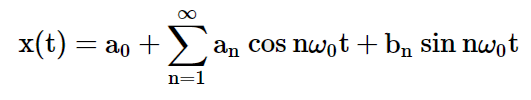
There is a lot of stuff going on in this equation and we will plot it in a minute. From an engineering perspective it is convenient to look at this representation as a function that has a dc and ac component.
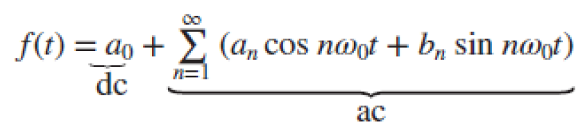
If you feel overwhelmed with the equation above, notice on how this representation resembles the equation for a sinusoidal function (below). The only difference is that we are summing a bunch of them rather than having just one.
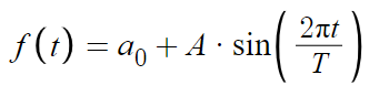
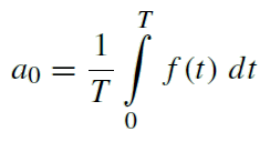
The coefficient from the dc component is is the average value of the waveform that can be directly evaluated from the waveform and is given by
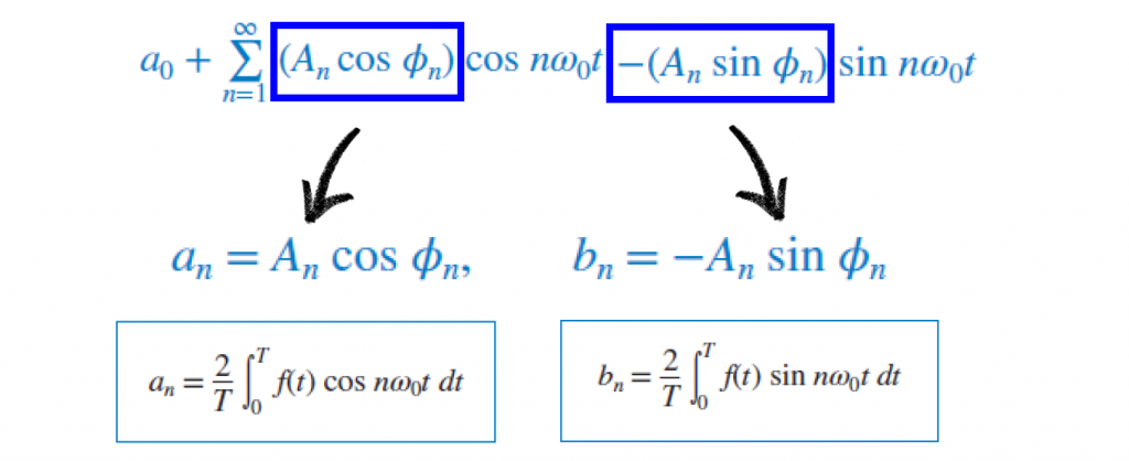
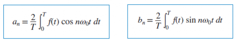
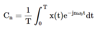
For the ac component, an and bn are called the Fourier coefficients and are defined as follow
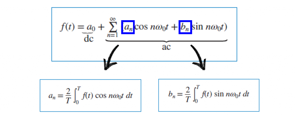
The Fourier coefficients, an and bn control the amplitudes of the two sinusoidal functions respectively.
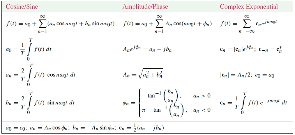
Fourier Coefficients Tables
The Fourier coefficients for the most common periodic signals are normally provided in tables. These tables can vary the way they present the coefficients, but at the end of the day, it is the same information. I am providing two tables examples below.
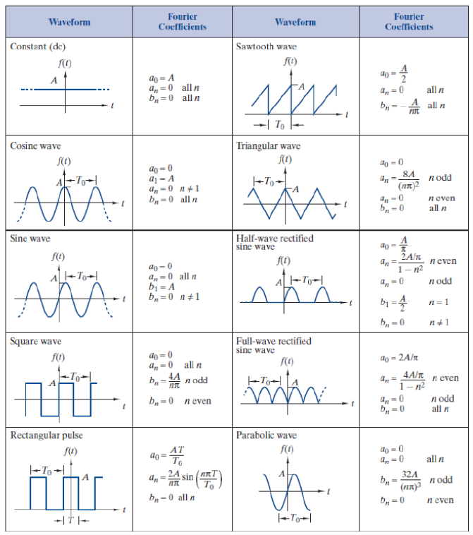
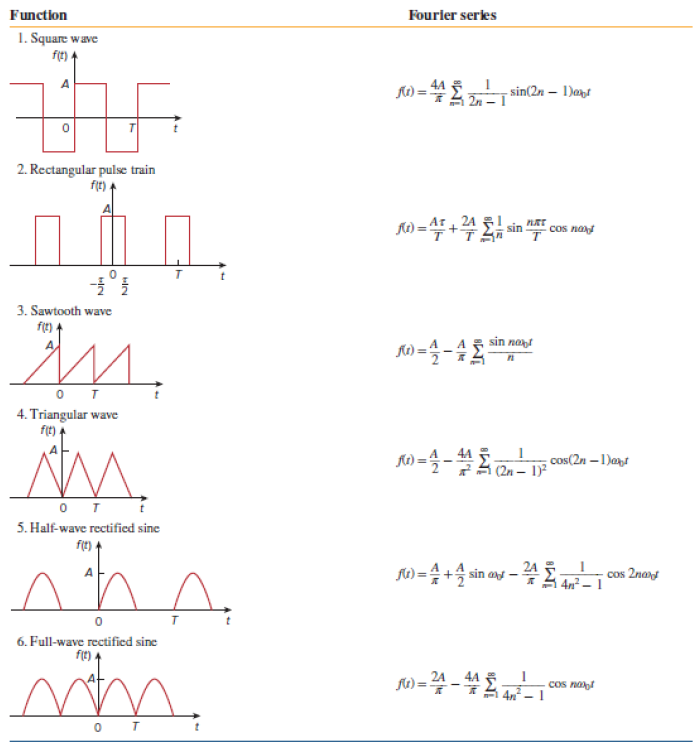
If your periodic signal is not on a table, you will need to find the Fourier coefficients by definition.
Let's plot the Fourier series for some of the most common used periodic functions. I am using the equations from Table 2 in the "Fourier Coefficient Tables" section above in GeoGebra.
Square Waveform (Live Animation)
Triangular Waveform (Live Animation)
Sawtooth Waveform (Live Animation)
Cosine Form
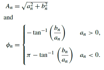
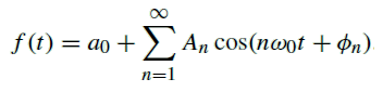
The trigonometric form of the Fourier series can be written in several alternative yet equivalent forms. We will start with the following statement: the sum of the sinusoids inside the sigma notation can be converted into a single sinusoid as follows.

where
Plot
We can use Desmos to validate this initial statement.
This results in the cosine representation with the coefficients in polar form.
Ptolemy’s Identity
From the cosine representation of the Fourier series and using the Ptolemy's identity...
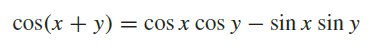
We get the following expression for the Fourier series:
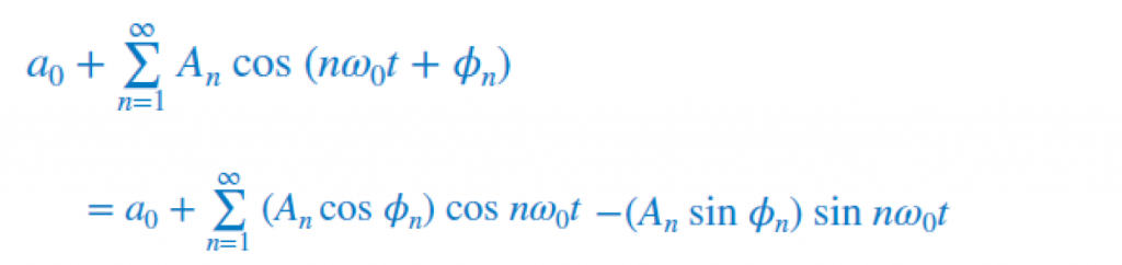
This results in a new expression for the Fourier coefficients.
Exponential Form
The exponential form of the Fourier series, also called Complex Fourier Transform, is the most complete form of all 3 forms described here. The trigonometric and cosine forms (also called Real Fourier Transforms) restrict the mathematics to real numbers, and that has the potential to restrict the description of how physical systems behave. In the world of mathematics, the complex Fourier transform is a greater truth than the real Fourier transform.
As engineers I believe we should be aware of which tool can solve the problem that you have in hands best. The complex Fourier transform can be overkill for certain topics in engineering. Nevertheless, understanding this last form allows you to communicate with professionals in the field, ability to understand books, papers, technical articles, etc.
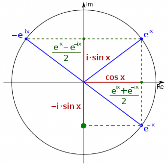
In the exponential Fourier series representation, the orthogonal functions are the exponential functions. To get to the final expression, we start from using the trigonometric relationship of the Euler's formula.
Note: if you are not familiar, or need a review on the Euler's formula, you can read it here.
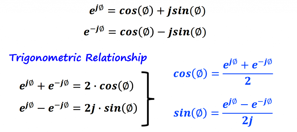
These relationships are key for the complex form of the Fourier series. The equations above relate complex numbers with ordinary sinusoids, which are present on the trigonometric form of the Fourier series. We can rearrange these equations a little bit.
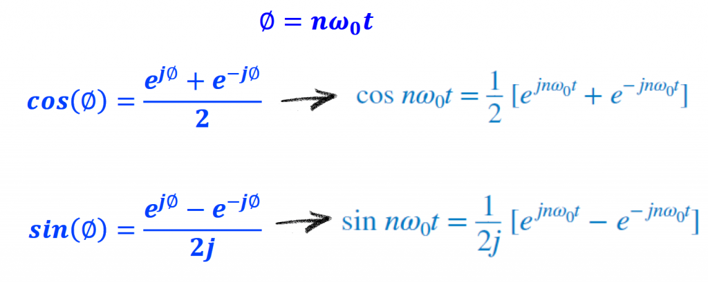
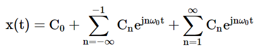
Each expression is the sum of two exponentials: one containing a positive frequency, the other containing a negative frequency. In other words, when sine and cosine waves are written as complex numbers, the negative portion of the frequency spectrum is automatically included. The positive and negative frequencies are treated with an equal status.
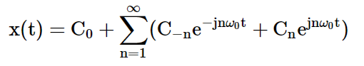
Substituting the equations above into the trigonometric form, we get the first equation for the complex form of the Fourier series.
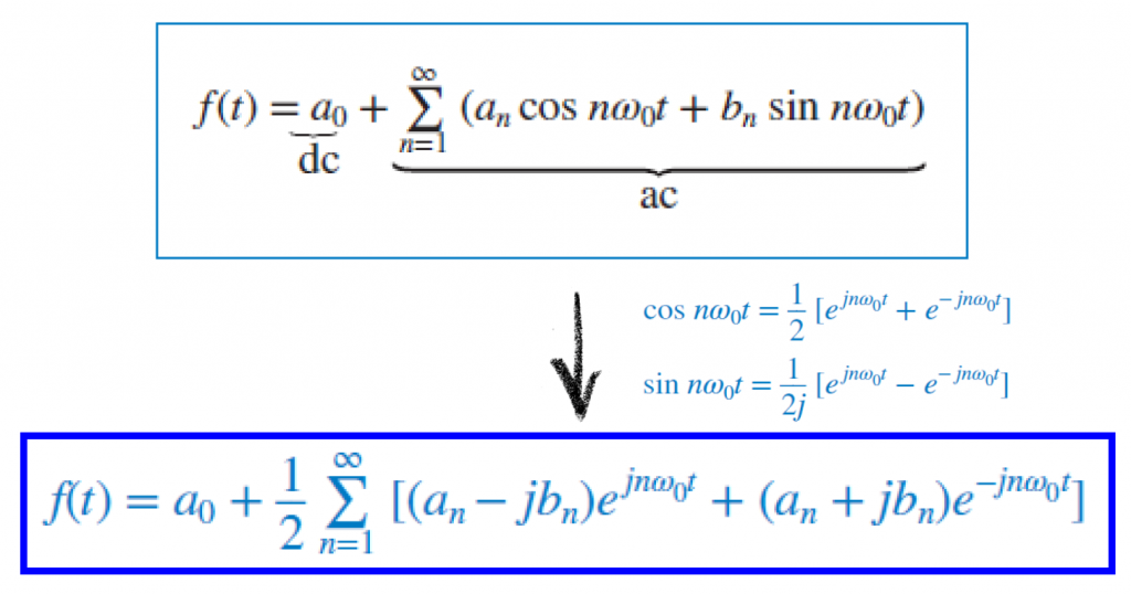
We are almost there. Notice that we have two terms in the equation that are the conjugate of each other.
Note: quick review, a conjugate of a complex number is another complex number which has the same real part as the original complex number and the imaginary part has the same magnitude but opposite sign.
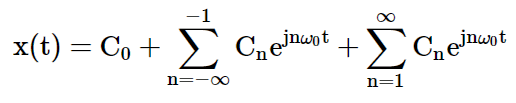
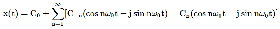
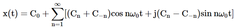
If we rewrite the complex numbers considering that conjugate...
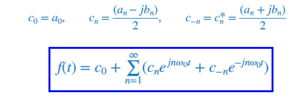
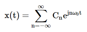
And in a more compact form, the famous exponential or complex Fourier transform.
Exponential and Cosine Coefficients Relationship
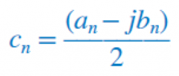
Some resources relate the exponential form to the cosine form as follow.
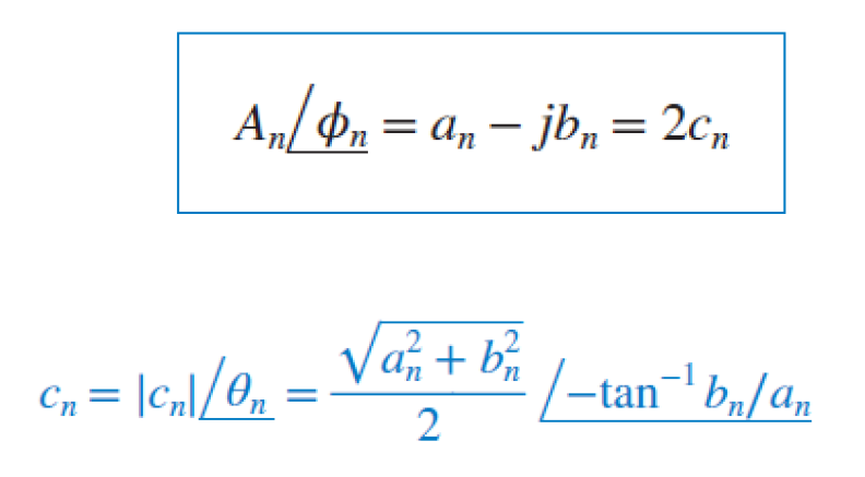
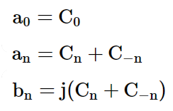
Exponential and Trigonometric Coefficients Relationship
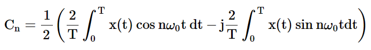
We can write the complex Fourier coefficient cn in terms of an exponential rather than the trigonometric Fourier coefficients, an and bn. This representation is going to be important to understand Fourier Transforms later.
Substituting an and bn into the cn equation:
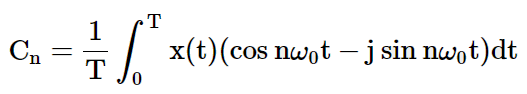
If we go to the complex plane, cos(x) - jsin(x) are the basis functions of the the vector e-ix .
With that we get the following exponential Fourier coefficient:
Summary
Dirichlet Conditions
To guarantee that a periodic function f(t) has a realizable Fourier series, it should satisfy a set of conditions known as the Dirichlet conditions.
Briefly, the Dirichlet-Jordan test states that if a periodic function f(x) has a finite variation during one period, then the Fourier series converges, as n → ∞ . In particular, if f is continuous at x, then the Fourier series converges to f(x).
In engineering applications, the Fourier series is generally presumed to converge almost everywhere (the exceptions being at discrete discontinuities) since the functions encountered in engineering are better-behaved than the functions that mathematicians can provide as counter-examples to this presumption.
Fourier Transform
The Fourier series is a perfectly suitable construct for representing periodic functions, but what about nonperiodic (or aperiodic) functions? This is where Fourier Transform comes in place to answer this question.
Note: Fourier Transform can be applied to periodic signals as well as aperiodic signals.
Fourier transform is a mathematical operation for converting a signal from time domain into its frequency domain.
Frequency Domain
We begin with the following pair of expressions:
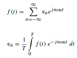
The complex coefficient can sometimes be represented with a different interval of integration (but still within one period).
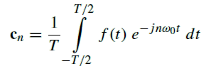
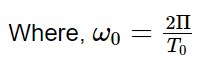
These two quantities form a complementary pair with f(t) defined in the continuous time domain and cn defined in the discrete frequency domain as nω0, with ω0 = 2π/T.
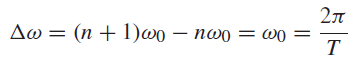
For a given value of T, the nth frequency harmonic is at nω0 and the next harmonic after that is at (n+1)ω0 . Hence, the spacing between adjacent harmonics is
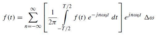
If we insert cn into the complex Fourier series, and replace 1/T with Δω/2π, we get
As T → ∞, Δω→dω and nω0 →ω, and the sum becomes a continuous integral:
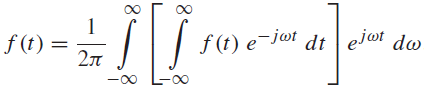
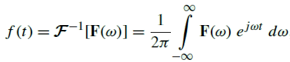
We arrive to the formal definitions for the Fourier transform F(ω) and its inverse transform f(t):
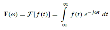
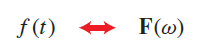
Occasionally, we also may use the symbolic form
Convergence of the Fourier Integral
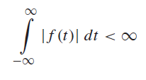
Not every function f(t) has a Fourier transform. The Fourier transform F(ω) exists if the Fourier integral given by
converges to a finite number or to an equivalent expression. As general rule, the Fourier integral does converge if f(t) has a no discontinuities (i.e., it is single-valued) and the integral of its absolute magnitude is finite (absolutely integrable). That is,
A function f(t) still can have a Fourier transform - even if it has discontinuities so long as those discontinuities are bounded (or finite). For example, the step function A u(t) exhibits a finite discontinuity at t=0 if A is finite.
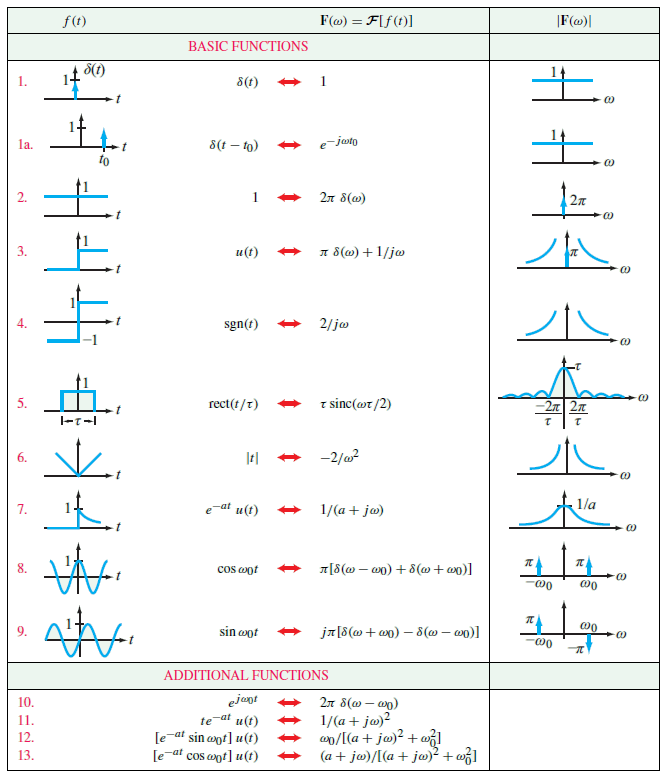
Fourier Transform Pairs
Below you can find a list of commonly used time functions together with their corresponding Fourier transform.
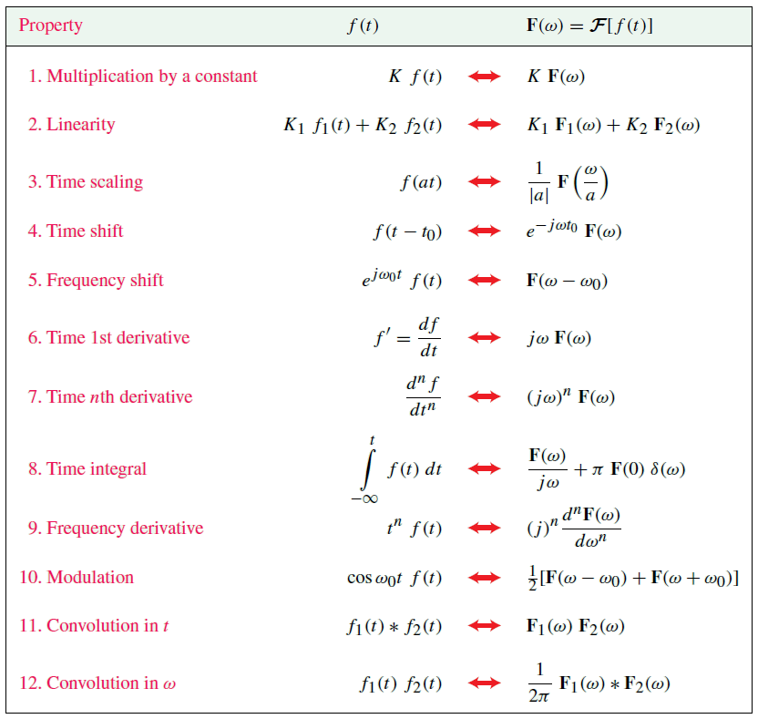
Fourier Transform Properties
To move back and forth between the time domain and the ω domain, we can use some useful properties of the Fourier transform.
Discrete Fourier Transform
soon

- Notation
- 3 Different ways to compute DFT
- Windowing
- Sizing
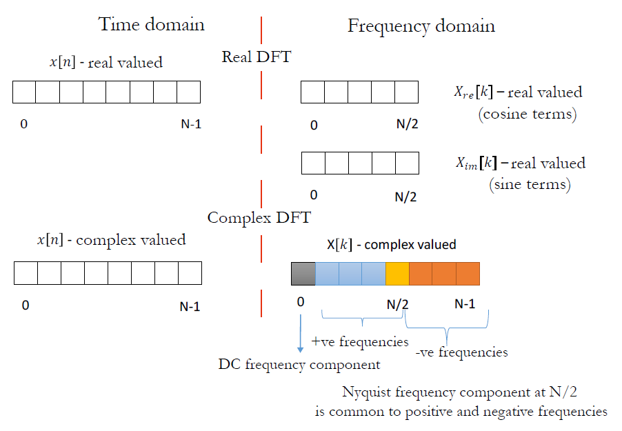
Real and Complex DFT
For each of the listed transforms presented so far, there exist a real and complex version. The real version of the transform comes from the trigonometric form, takes in a real numbers and gives two sets of real frequency domain points - one set representing coefficients over cosine basis function and the other set representing the coefficients over sine basis function.
The complex version of the transform represent positive and negative frequencies in a single array. The complex versions are flexible, that it can process both complex valued signals and real valued signals.
Epicycles with Fourier Series
There is a good chance that you probably have already seen some contents online using Fourier series to draw pictures like the one below. What is the connection between Fourier series and epicycles?
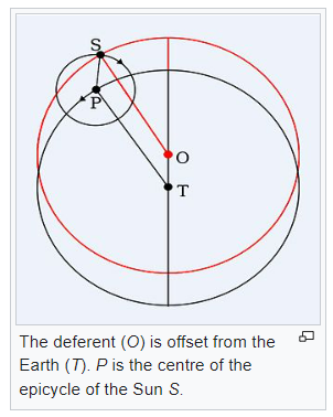
What is an Epicycle
An epicycle was a geometric model used to explain the variations in speed and direction of the apparent motion of the Moon, Sun, and planets.
Interesting enough, we can manipulate the way that we visualize the Fourier series to get a similar result to epicycle rotations.
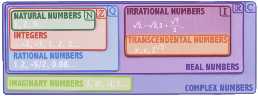
Real and Complex Exponential Signals
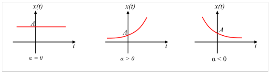
The first important concept to understand is the difference between an exponential function represented in the real numbers domain (

An exponential function, x(t) = Aeαt , with a real argument α, behaves in the following manner as we change the argument α.
The rotation comes when we represent the argument of the exponential function as a complex number
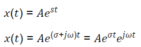
For the topic of Epicycle we can set σ=0, and we are left with the complex exponential function.
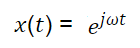
Applying Euler's formula (ejωt=cos(ωt)+jsin(ωt))
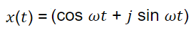
Plotting this function in the complex domain, where x = cos(ωt) and y = sin(ωt), we get a rotation (black point below).
In the real domain (
Fourier with Real Circles
To visualize x(t) = ejwt in the real domain (
Since the complex plane is “borrowing” the axis of the real domain (
Exponential and Trigonometric Forms Relationship
Before connecting the Fourier series with Epicycles (or more circles), it will be interesting to connect the exponential and trigonometric forms of the Fourier series together. Let's start with the exponential form.
If we unroll the equation above, we get the following...
We can use the visualization below to help us represent the exponential functions (vectors) with basis functions (sin and cos functions).
It is easy to get to this point and get confused, mainly because the result looks very similar to the trigonometric form of the Fourier series.
And in fact, it is the same. The only difference is that we can write the Fourier coefficients as complex numbers.
From the "Real and Complex Exponential Signals" section above, we saw that we can plot complex exponential functions in the real domain R by setting x = cos(ωt) and y = sin(ωt). The cosine and sine functions are present in both the exponential and trigonometric form, and from an Epicycles with Fourier series perspective, it doesn't matter which one you consider.
Fourier with More Circles
Let's bring back the exponential and trigonometric Fourier series equations.
I hope at this point, I convinced you that we can either use the exponential or trigonometric form for this Epicycles topic. As long as we set x = a cos(nωt) and y = b sin(nωt), we will be able to draw circles in the complex domain (
\left( a_{n},b_{n} \right)
=
\left( \left[ c_{n}+c_{-n} \right], j\left[ c_{n}-c_{-n} \right]\right)
=
\left( a,jb \right) = a+jb
Constant values of a and b
Let's start plotting the Fourier series with the circles, and for simplicity, let's consider the following:
- a0 = 0
- a = b = 1 for all circles
- use Re{x(t)} → cos(nωt) for the plot in the real domain (
Hopefully this can help visualizing what is happening in both domains at the same time.
One Circle (Live Animation)
Circles: c1 = cos(ωt) + j sin(ωt)
Complex Domain (
Real Domain (
Two Circles (Live Animation)
Circles: c1 = cos(ωt) + j sin(ωt); c2 = cos(2ωt) + j sin(2ωt)
Complex Domain (
Real Domain (
Three Circles (Live Animation)
Circles: c1 = cos(ωt) + j sin(ωt); c2 = cos(2ωt) + j sin(2ωt); c3 = cos(3ωt) + j sin(3ωt)
Complex Domain (
Real Domain (
I hope it is clear how the drawings are being generated. I think we are in good shape to start changing a and b.
Variable values of a and b
Now we are going to consider the following:
- a0 = 0
- circles will have their individual a's and b's
- use Re{x(t)} → cos(nωt) for the plot in the real domain (
Two Circles (Live Animation)
Circles: c1 = a1cos(ωt) + j b1sin(ωt); c2 = a2cos(2ωt) + j b2sin(2ωt)
Complex Domain (
Real Domain (
By controlling the a's and b's individually, we can start drawing different shapes in the complex domain. On the other hand, in the real domain (
If we add phase changes into the picture, we are going to create new shapes
Variable Phases (Live Animation)
Circles: c1 = a1cos(ωt + d1) + j b1sin(ωt + d1); c2 = a2cos(2ωt + d2) + j b2sin(2ωt + d2)
Complex Domain (
Real Domain (
More Variable Phases (Live Animation)
Circles: c1 = a1cos(ωt + d1) + j b1sin(ωt + d2); c2 = a2cos(2ωt + d3) + j b2sin(2ωt + d4)
Complex Domain (
Real Domain (
The last thing to cover here is just the rendering of the circles while they are rotating. Until now, I have been showing the exponential complex functions centered with the main circle in black. For simplicity, I am going to focus on an example with just 2 complex exponential functions (green and orange vectors below).
What we can do is to have the first exponential (in green) centered with the black circle, the next exponential (in orange) centered to the green point, and the final result (blue point) attached to the end of the orange circle.
If we control the amplitude of the second complex exponential function according to whatever value we want, it will start looking like the Epicycles graphs.
The result coming out of this rendering is exactly the same as the one with all complex exponential functions aligned with the black circle.
Ultimately, you can apply exactly the same rendering concept for all the desired complex exponential functions that you want from the Fourier Series and we will get the famous Epicycles animation.
Render Images
We are almost there. Hopefully the last section showed that all we need to draw shapes is to control the amplitudes, frequencies and phases of the different cosines and sines while plotting them in the complex domain as x and y coordinates respectively. The circles can be arranged in a way that they will look like Epicycles.
To draw an image with with these circles, all we need to do is to treat the image as a function and find the respective Fourier coefficients, and then pass those coefficients to the x and y coordinates and render the image back on the screen.
There are several examples online that explain this process or have interactive animations that you can have fun with. I will leave some links below that you can potentially explore.
- How to create images in Desmos using Epicycles and Fourier Series [reddit] (Link)
- Drawing with Fourier Transform and Epicycles [YouTube] (Link)
- Fuyye Series and Making Sound from the Image [Article] (Link)
- A Tale of Math & Art: Creating the Fourier Series Harmonic Circles Visualization [Article] (Link)
- An Interactive Guide to the Fourier Transform [Article] (Link)
The Desmos rendering code below, allows you to introduce Fourier coefficients with circle parameters: amplitude (rc), frequency (vc), and phase (ac). You can play with some random values or plug values from an image conversion.
References
- [Ref 1] “Chapter 8: The Discrete Fourier Transform”, The Scientist and Engineer's Guide to Digital Signal Processing By Steven W. Smith [Book Chapter]
- [Ref 2] “Chapter 31: The Complex Fourier Transform”, The Scientist and Engineer's Guide to Digital Signal Processing By Steven W. Smith [Book Chapter]
- [Ref 3] “Circuit Analysis and Design”, Fawwaz T. Ulaby, Michel M. Maharbiz, and Cynthia M. Furse [Book]
- [Ref 4] “Intuitive Guide for Fourier Analysis and Spectral Estimation”, Charan Langton and Victor Levin [Book]
- [Ref 5] “Digital Modulations using Python”, Mathuranathan Viswanathan [Book]
Interactive Websites
- [Ref 6] “An Interactive Introduction to Fourier Transform”, Jez Swanson Website [Interactive]
- [Ref 7] “Drawing with Fourier Series”, olgaritme Website [Interactive]
- [Ref 8] “myFourierEpicycles”, Tony Rosler Website [Interactive]
YouTube Videos
- [Ref 9] “Epicycles, complex Fourier series and Homer Simpson's orbit”, Mathloger [Video]
- [Ref 10] “What is a Fourier Series? (Explained by drawing circles)”, SmartEveryDay [Video]
- [Ref 11] “But what is a Fourier series? From heat flow to drawing with circles”, 3Blue1Brown [Video]
Other Resources
- [Ref 12] “Relation between Trigonometric & Exponential Fourier Series”, TutorialsPoint Website [Article]
- [Ref 13] “Signals and Systems: Real and Complex Exponential Signals”, TutorialsPoint Website [Article]