Euler’s Formula
There are several resources online that cover this subject with more detail that what I am providing here, but the goal with this article is to give a quick introduction to this topic and provide the fundamental knowledge behind it. If you are looking for more detail, or this article doesn't suite your learning style, you can check the References section below and hopefully they can help with your learning.
Taylor Series
The reason why I start with describing Taylor series is because Euler used this mathematical tool to reach to the famous Euler's formula.
In mathematics, the Taylor series is used to describe functions using an infinite sum of terms that are expressed in terms of the function's derivatives at a single point.
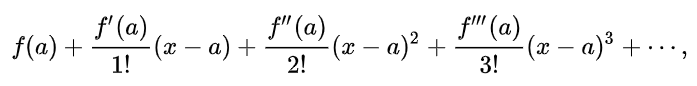
where n! denotes the factorial of n. You can sometimes see this expression written in a more compact notation, called sigma notation (meaning as a summation of many similar terms).
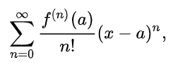
where f(n)(a) denotes the nth derivative of f evaluated at the point a.
Note: When a=0, the series is also called a Maclaurin series.
We can use Desmos to visualize this Taylor series concept. I am applying the first expression of the Taylor series up to the 20th derivative to a sine function. You can move x0 around, that represents the point a, and you can add or remove terms from the series by moving D.
Note: Don't be afraid to modify/add/remove Desmos functions and parameters. Feel free to modify whatever you want, have fun with it. You can always reload the page to go back to the initial state.
On a side note, there are other ways to describe functions on a specific point besides Taylor series. For example, Padé Approximant performs better near a specific point by a rational function of given order. There is a wonderful video about this topic here -> Padé Approximants [YouTube Video]
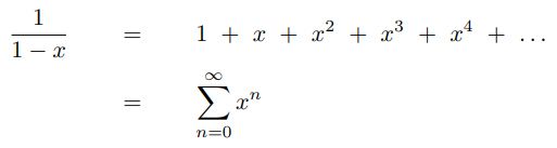
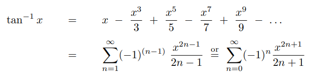
Commonly Used Taylor Series
Below you can find the most common used Taylor Series. We will be using a couple of them soon.
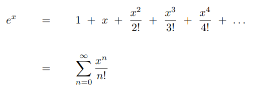
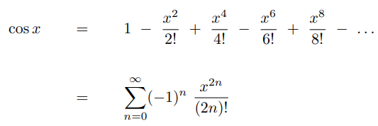
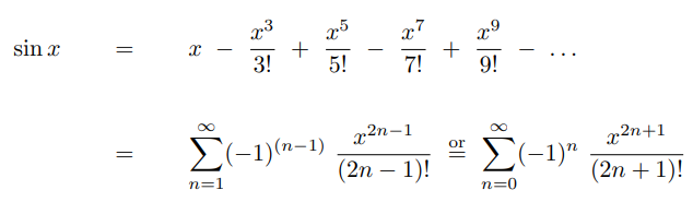
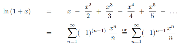
Taylor Series Applied to Complex Functions
Around 1740 Leonhard Euler was focusing his work towards the complex plane, and in 1748, in his foundational work "Introductio in Analysin Infinitorum", Euler introduce the formula named after him for the first time. Euler compared the series expansion of the exponential and trigonometric expressions in the complex plane.
If we take the exponential of an imaginary number and write it out as a series expansion, we get
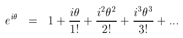
Notice that all we are doing is using the Taylor series from the previous section and substituting x by iθ. Also note that i2=-1 and i3=i2· i=-i and similarly for higher powers of i we get
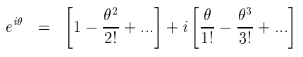
Interesting enough, applying the substitution of x by θ to the two trigonometric functions, cosine and sine, we get
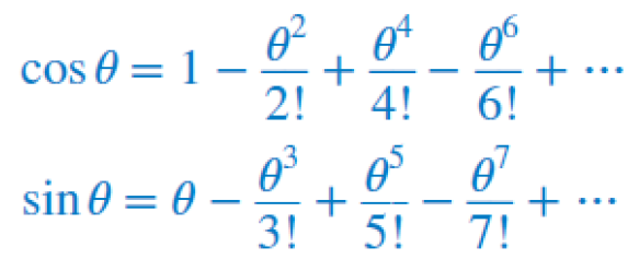
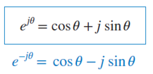
Comparing the exponential function with the trigonometric functions we can see that
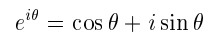
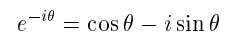
Which is known as Euler's formula. Similar expansions for e-iθ give the identity
Eurler's Formula
The Euler's formula is telling us that an exponential function in the complex domain is composed by two orthogonal functions, sine and cosine.
If we plot them over time in the complex domain, we get the animation below. The real part of the formula varies as a cosine function, and the imaginary part of the formula varies as a sine function.
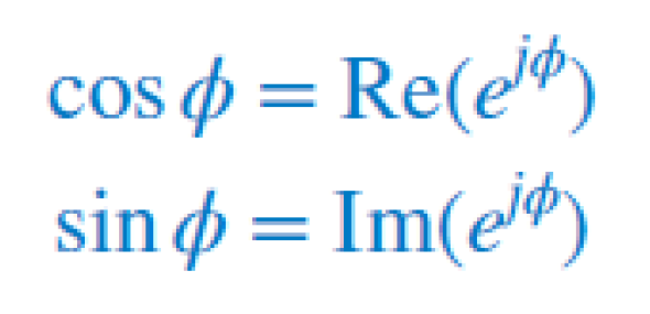
Some resources represent these basis functions in the complex plane with the expressions below.
Curiosity
The sine and cosine are orthogonal 2D projections of the 3D Unit Helix (the Unit Circle rotated through spacetime).
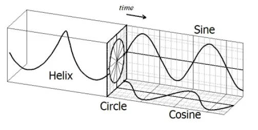
(Live Animation)
Trigonometric Relationship
There a couple of trigonometric relationships for the Euler's formula that are useful to know, and the reason behind it is because they are used with one way of writing the famous Fourier Series.
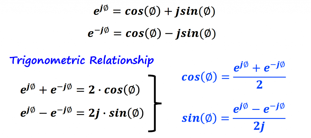
Note: This result is extremely important, we have developed a way of writing equations between complex numbers and ordinary sinusoids.
We can actually visualize these relationships if we use the complex plane to represent them. If we see ejθ and e-jθ as vectors, cos and sin can be obtained by summing and subtracting these vectors respectively. Don't forget to divide the result by 2 on both operations.
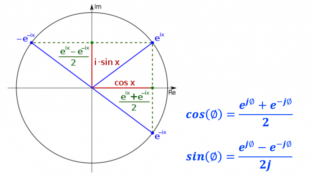
If it is hard to visualize these vectors subtraction and addition from the picture above, I will leave a link to an animations to help with that.
Move point C around to position vector v (in blue) and observe the resultant vector a (in green) to validate the equations above.
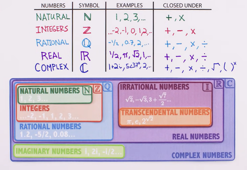
Complex Numbers Review
Welch Labs - Imaginary Numbers are Real (Videos)
- Part 1. Introduction (Link)
- Part 2. A Little History (Link)
- Part 3. Cardan’s Problem (Link)
- Part 4. Bombelli’s Solution (Link)
- Part 5. Numbers are Two Dimensional (Link)
- Part 6. The Complex Plane (Link)
- Part 7. Complex Multiplication (Link)
- Part 8. Math Wizard (Link)
- Part 9. Closure (Link)
- Part 10. Complex Functions (Link)
- Part 11. Wandering in Four Dimensions (Link)
- Part 12. Riemann's Solution (Link)
- Part 13. Riemann Surfaces (Link)
Additional Resources
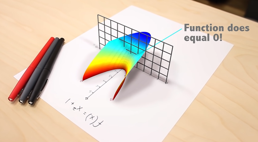
On the videos above, the author plots the graph below where you can see the solutions of a quadratic function with imaginary roots. There is a cool animation on GeoGebra (Visualizing Complex Roots of Quadratic Equations) that you can use to vary this function and get a better insight of the roots of quadratic equation.
References
Complex Numbers
- [Ref 1] “Imaginary Numbers are Real - PDF”, WelchLabs Website [Resources]
Taylor Series
- [Ref 2] “The Most Important Math Formula for Understanding Physics”, Physics with Elliot [Video]
- [Ref 3] “Taylor Series”, 3Blue1Brown [Video]
Euler Formula
- [Ref 4] “What is Euler's formula actually saying”, 3Blue1Brown [Video]
- [Ref 5] “Euler's Formula”, Wikipedia [Article]
- [Ref 6] “Euler's Formula”, Numberphile [Video]
- [Ref 7] “Intuitive Understanding Of Euler’s Formula”, Better Explained [Article]