Angle Modulations
This article focus on analog angle modulations: Phase Modulation (PM) and Frequency Modulation (FM).
Note: The article combines mathematical expressions with visuals with the goal to help understanding the concepts from different perspectives. The goal by presenting math equations is not to overwhelm the reader but rather an attempt to connect the theory with the practical world.
Angle Modulation
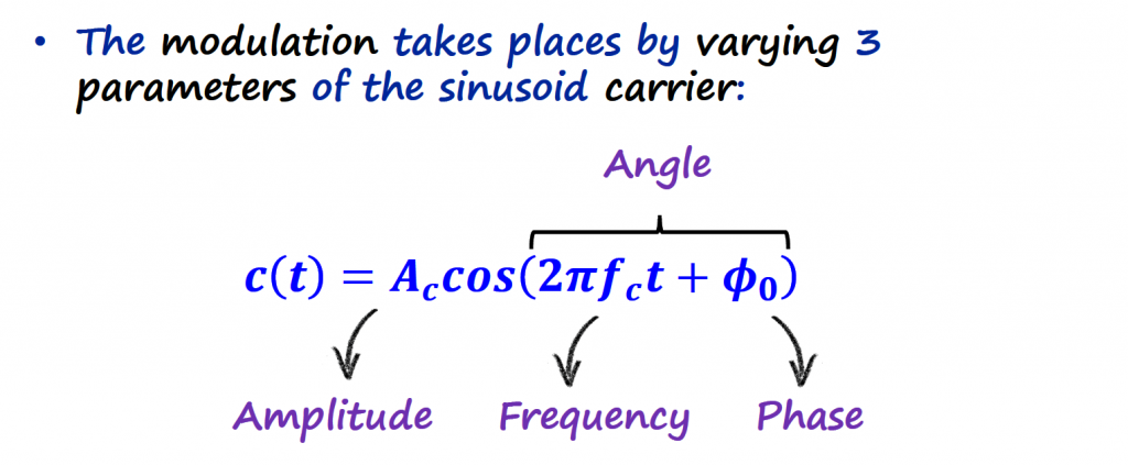
In AM signals, the amplitude of a carrier is modulated by the information signal (m(t)), and hence, the information content of m(t) is in the amplitude variations of the carrier (c(t)). The other two parameters of the carrier sinusoid, namely, its frequency and phase, can also be varied linearly with the information signal to generate frequency-modulated and phase-modulated signals, respectively.
Phase Modulation (PM)
Phase modulation is probably the easiest modulation to understand, compared with FM modulation.
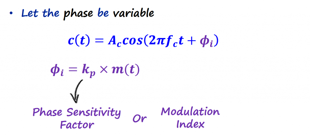
The information signal (m(t)) is now part of the phase of the carrier (c(t)). The constant value (kp) is called modulation index, and it can be used to regulate the amplitude of m(t).
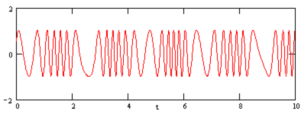
If the information signal (m(t)) is an analog signal, the phase changes are gradual and not obvious.
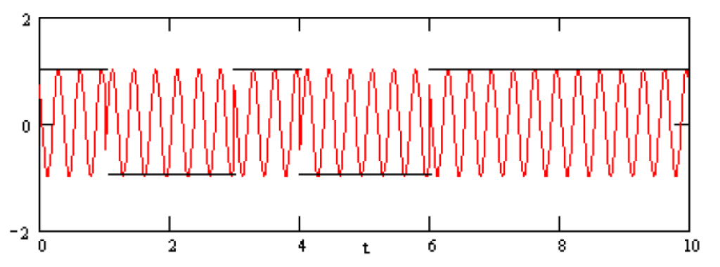
On the other hand, if the information signal (m(t)) is a digital signal, the phase changes are discrete.
The Desmos animation below can help with visualizing the phase changes for different types of information signals (m(t)). The green line is the carrier and you can turn on and off any of the 3 signals to modulate the carrier's phase accordingly.
Notice on how the square waveform (which is equivalent to digital data), produces phase changes that are more visible than using the triangle waveform.
On the Desmos animation above, I kept the information signals turned off so we could visualize the phase changes without too many distractions. However, if I superimpose (visually) the information signal (m(t)) with the modulated carrier (green waveform), we can get more insight on what is actually happening.
Analog PM is not that useful, since the changes in phase are smooth, it makes it harder to recover the information and needs more complex receivers.
On the other hand, digital PM is widely used for digital data modulation. Since this article is focusing on analog modulations, you can check the article under the section "PSK Modulation" for more information about digital PM.
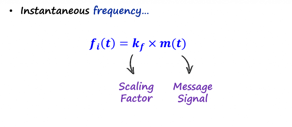
Instantaneous Frequency
The math from this point on can be a bit intimidating at first, but we need to understand the concept of instantaneous frequency before spending time with analog FM modulation.
FM signals vary the instantaneous frequency in proportion to the information signal (m(t)). This means that the carrier frequency is changing continuously at every instant. At first glance this doesn't make much sense, since to define a frequency, we must have a sinusoidal signal at least over one cycle (or half-cycle or a quarter-cycle) with the same frequency.
One way to digest this concept of instantaneous frequency, is to relate to the understanding of instantaneous velocity. Until the presentation of derivatives by Leibniz and Newton, we were used to thinking of velocity as being constant over an interval, and we were incapable of even imagining that velocity could vary at each instant. Similar experience can happen with respect to instantaneous frequency.
Knowing the concept of derivatives make our life easier to find an equation for the instantaneous frequency. Briefly, it is easier to understand that we can compute linear velocity by measuring two positions at different times and subtract them, which in essence is doing a derivative of the position over time. The same steps can be taken with angular positions to find angular velocity.
What I like about the animation above, is the fact that we can represent the same concept with two different views. We will focus on the graph with the blue dot for now. That graph shows a circular motion, and from that graph the angular velocity is how fast that blue dot is moving around the circular path. We can find that angular velocity by subtracting two angular positions over time.
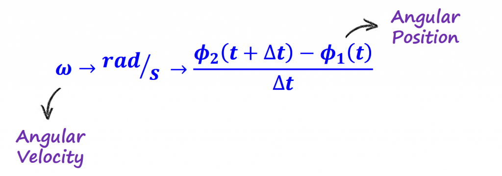
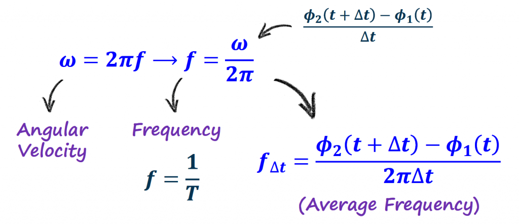
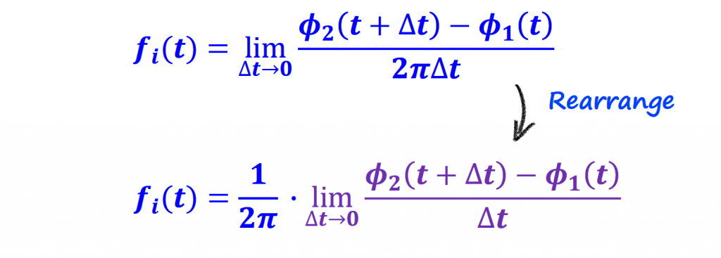
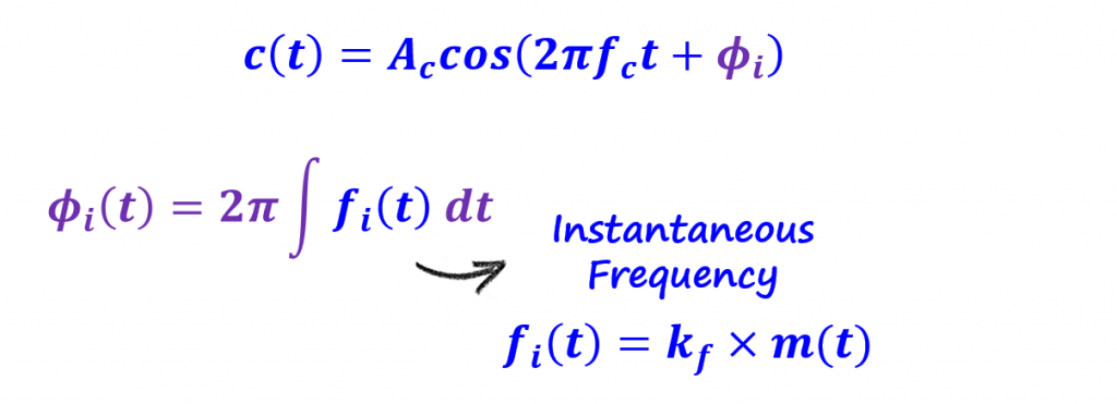
To find the instantaneous angular velocity, we can use the derivative and relate that derivative to frequency.
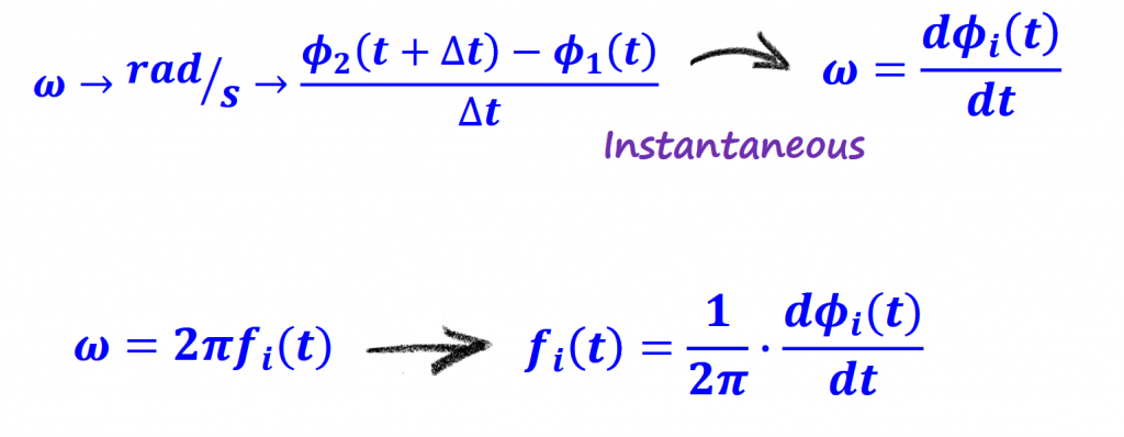
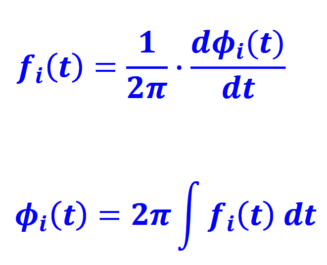
Voila, you get the expression for the instantaneous frequency, and we can manipulate that equation and write it in terms of angular position too. Keep those two equations below in mind, we will be using them later.
In case you want a more visual way to explain the instantaneous frequency, read the section below. Otherwise, you can skip this section.
Visual Interpretation of Instantaneous Frequency
Let's go back to the point were we had the relationship between angular velocity and angular position.
From here, if we relate angular velocity with frequency, we can find the equation for the average frequency.
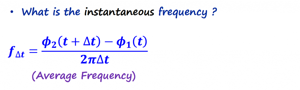
If we represent the average frequency on the graph that had the blue dot (circular motion), the average frequency is the path (in green) that the blue dot does over the full circle (2π). Instantaneous frequency in that path will be the small blue dot at that particular instance of time.
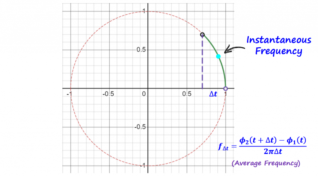
To find the value of the small blue dot, we need to make the time interval very small (ideally to zero). That is equivalent to find the limit of the average frequency when the time interval goes to zero.
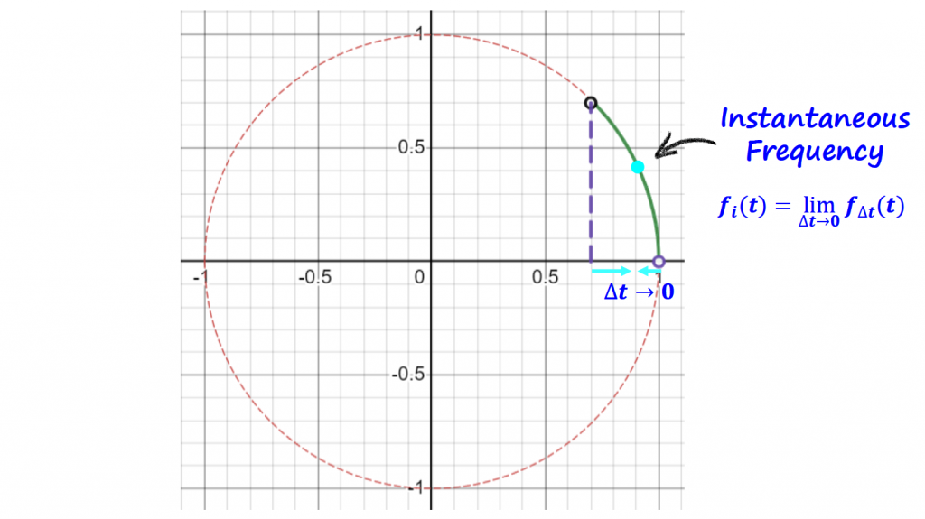
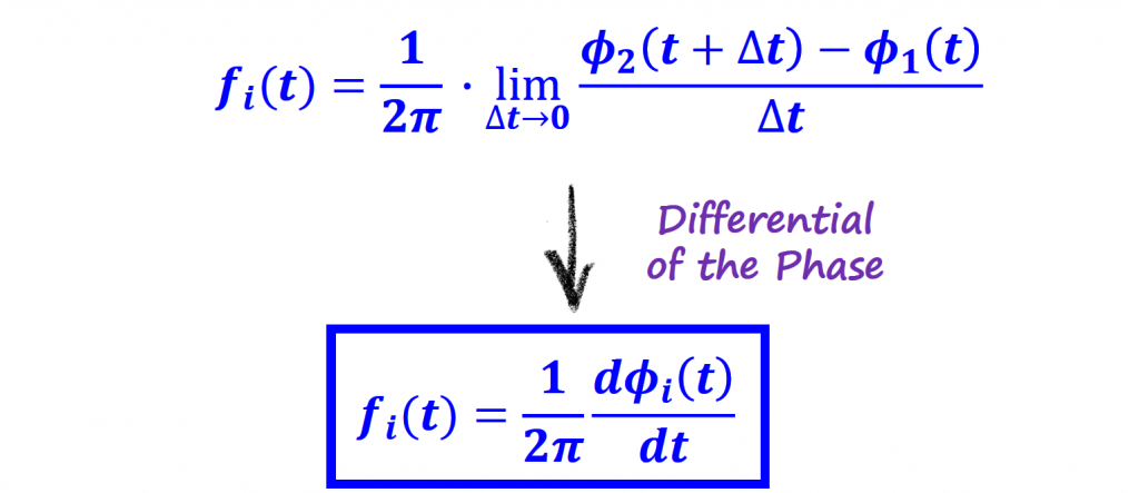
At this point, you might think that you are stuck with the limit but in fact, that limit is the definition of a derivative.
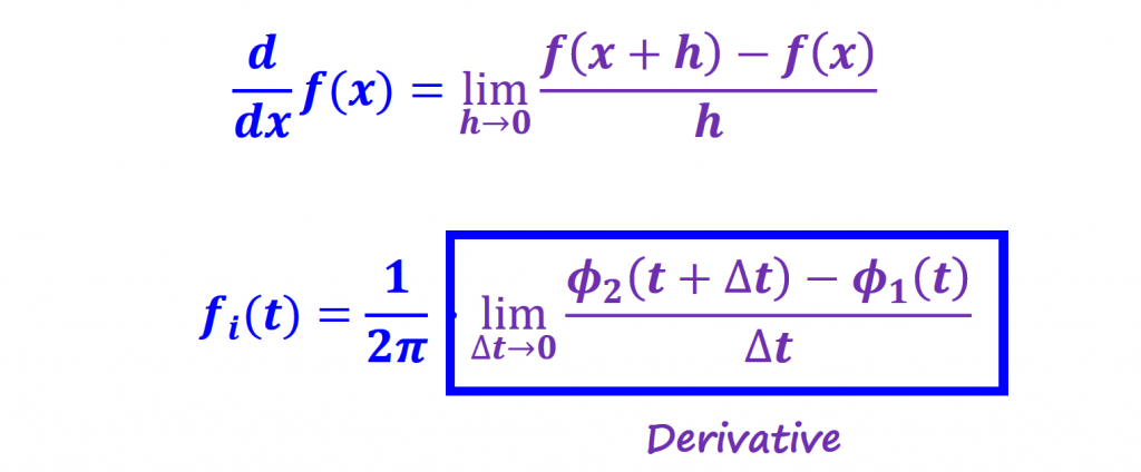
And we get the same expression for the instantaneous frequency.
Another concept that we need to start being comfortable with from this point on, is the fact that we can have positive and negative frequencies.
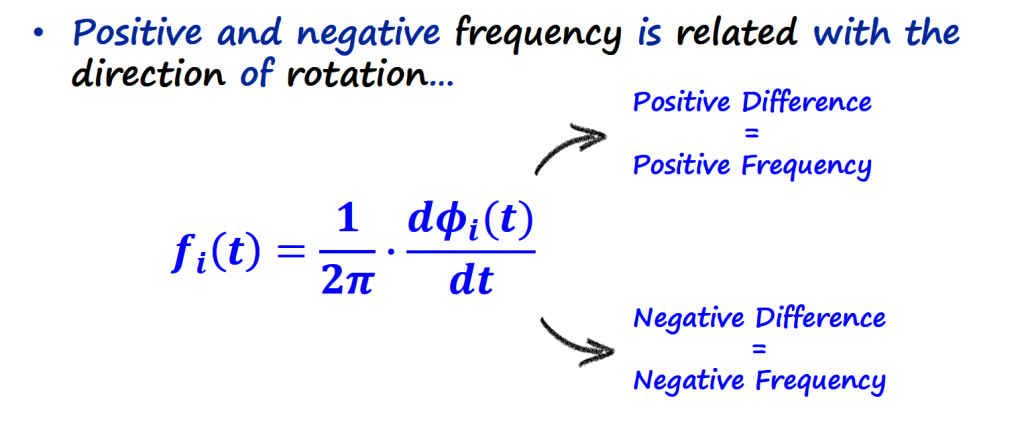
We can see this in action using GNURadio.
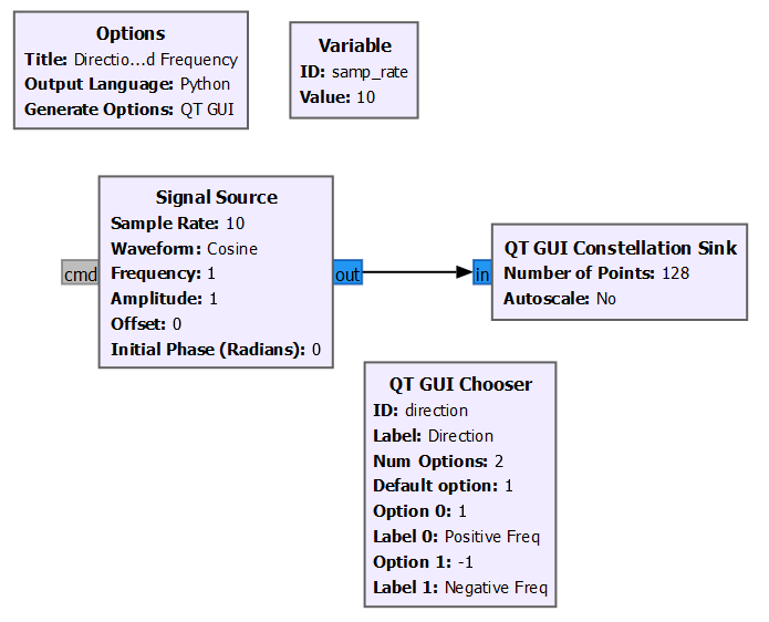
Having positive and negative frequencies correspond to have those IQ values rotating counter clock and clock wise respectively.
Frequency Modulation (FM)
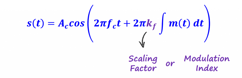
FM modulation is a variation of angle modulation. For FM we are modulating the instantaneous frequency with the information signal (m(t)). We need to rearrange the carrier equation to include the instantaneous frequency. This is where the instantaneous frequency equation and respective angular position equation derived in the previous section comes handy.
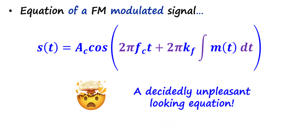
Analog FM is one of the more complex ideas in communications. It is very difficult to develop an intuitive feeling for it. We are going to give it a shot under the Analog FM section.
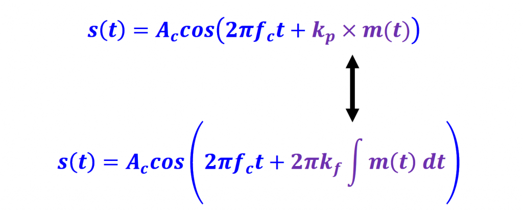
PM <-> FM
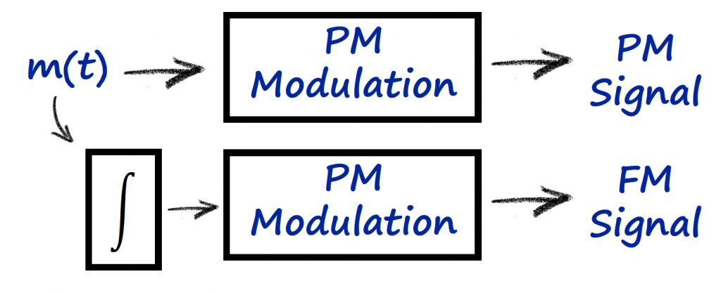
In certain situations it might be convenient to use only a PM or FM modulator and still be able to modulate signals with any angle modulation technique. Notice below that we can either integrate or derive the message (m(t)) to go between PM to FM and vice versa.
PM to FM Modulation
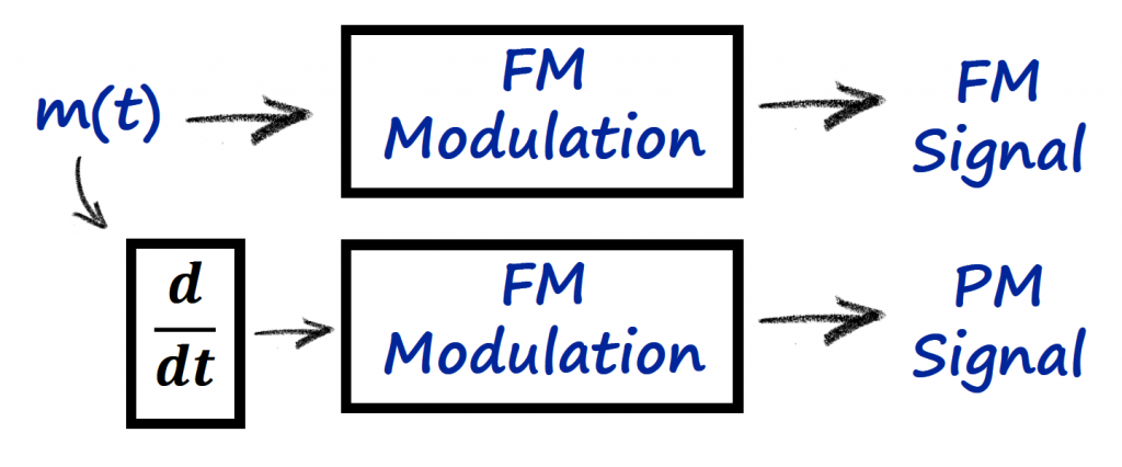
FM to PM Modulation
Analog FM
Despite analog FM being a complex idea in communications, we are still going to develop an understanding of it. The reason behind it is because a good portion of radio transmission are analog FM and when the digital version of the FM modulation (FSK) is covered, this knowledge will be very useful too.
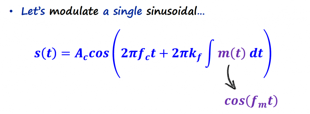
To help with that understanding we are going to make things easier to analyze for now. We are going to consider a simple cosine waveform as the information signal (m(t)) to transmit.
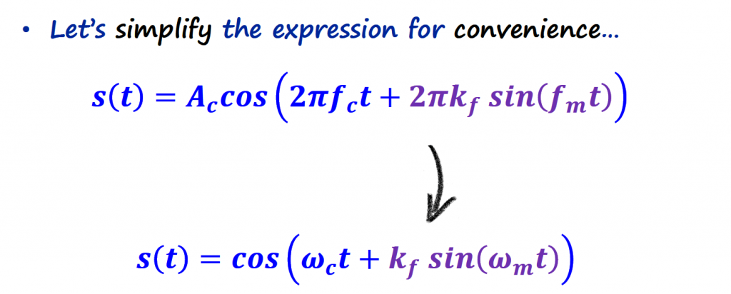
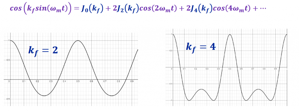
For simplicity, we make Ac = 1, and we absorb 2π into the scaling factor (kf). Let's expand the cosine function using a trigonometry identity.
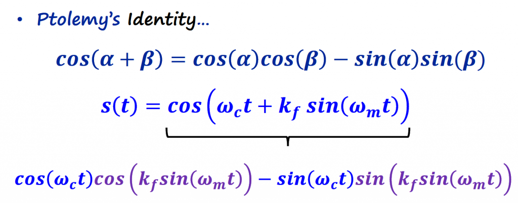
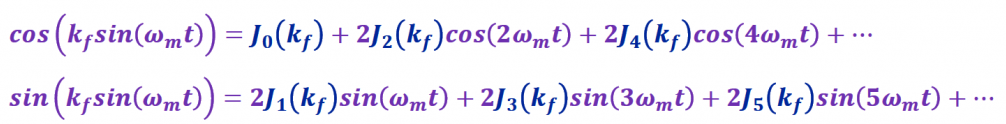
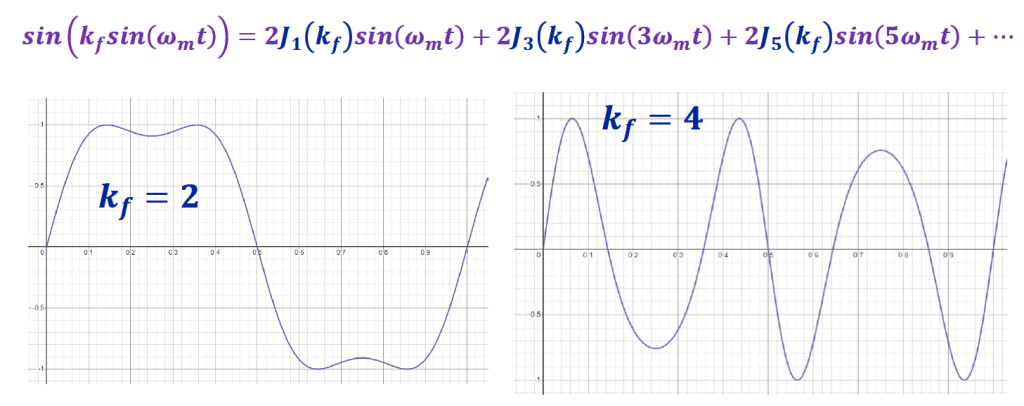
From here things start to become a bit scary. We can tackle this equation by expanding the sinusoidal functions that have the scaling factor in it.
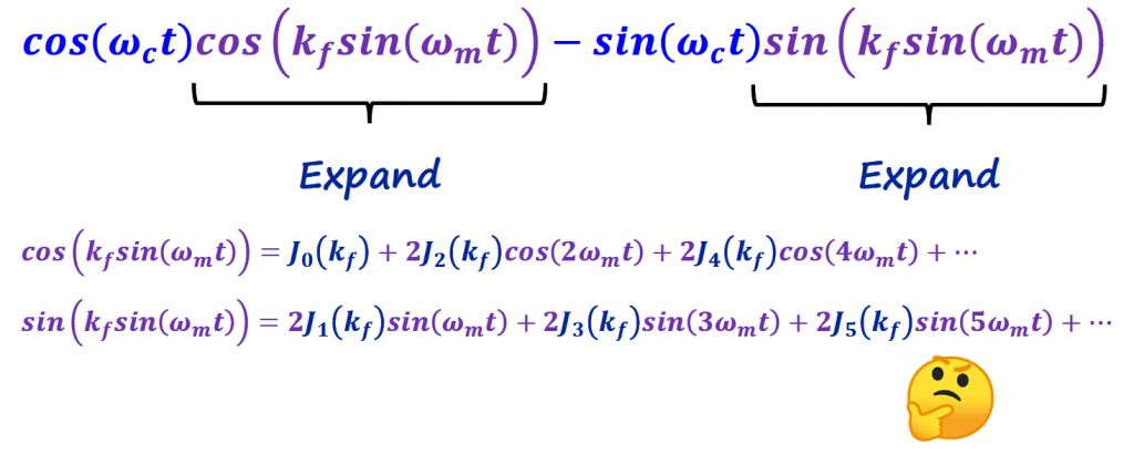
If you don't recognize the result of expanding the sinusoidal functions, don't panic. The J0, J1, J2, J3, J4, J5, etc... are what is called Bessel functions of the first kind. You can find more information about this expansion on this link. They are presented by Abramowitz and Stegun on the "Handbook of Mathematical Functions" (Link), page 113, equations 9.1.42 and 9.1.43.
For this particular case, it seems that these Bessel functions are shaping the amplitude of a bunch of sinusoidal functions.
Bessel Functions
Bessel functions are the solutions of the Bessel differential equation (a variable coefficients linear second order ODE). Jα and Yα are the Bessel functions of the first and second kinds.
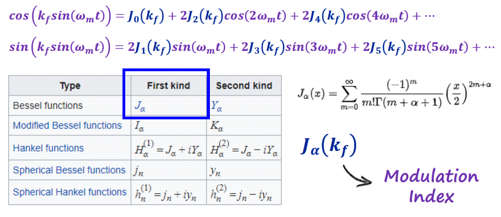
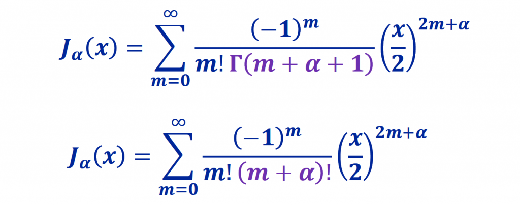
Bessel functions of the first kind can be defined by its series expansion...
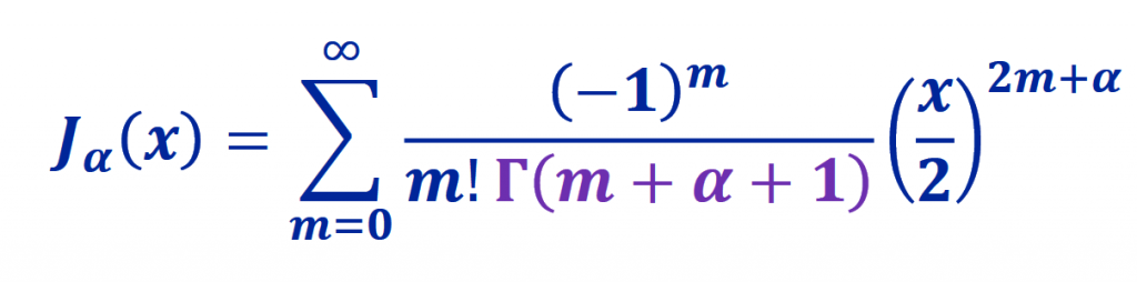
There is a lot of going on in this equation, and to make things easier, it would be nice to plot this equation.
Let's go step by step here...
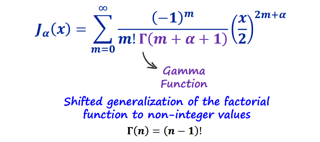
The first thing to do, is to understand what the Gama function is. Briefly, the gamma function (Link) interpolates the factorial function to non-integer values. In other words, it is a way to find smooth curves that connect points given by that factorial equation.
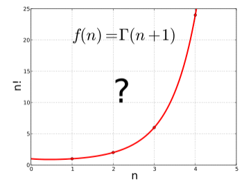
We substitute the Gama function by the factorial equation...
Now we are in good shape to plot some of these Bessel functions of first kind. Let's use Desmos to plot the first 4 Bessel functions.
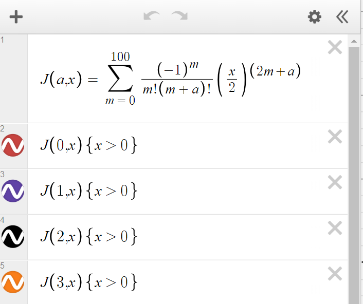
We get more sinusoidal functions. But what we are interested in is the value of those functions for particular scaling factors (kf).
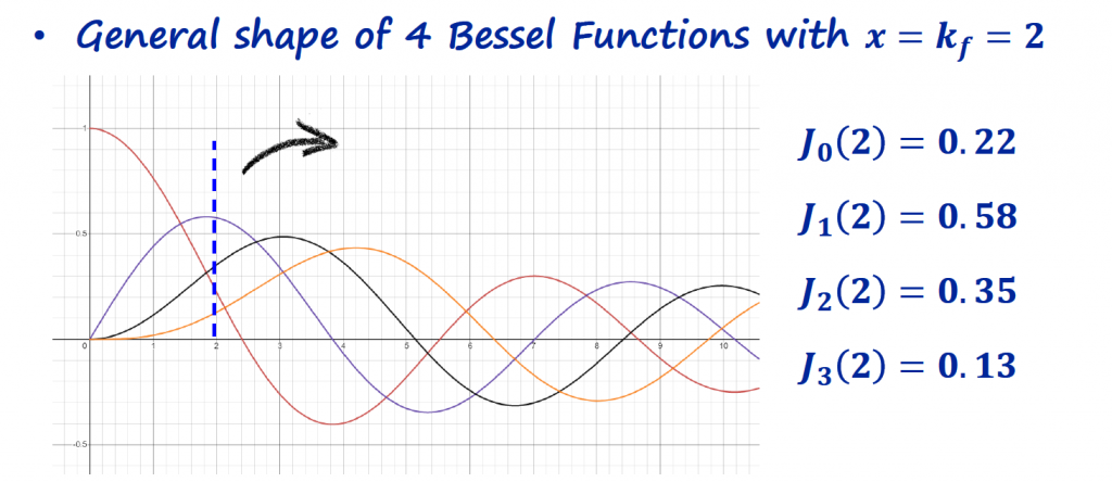
If we compute and plot the equations that we just expanded and substitute the Bessel equations of first kind for their respective value at different scaling factors (kf), we get the following plots:
We observe that the Bessel functions are modulating the amplitude on different sinusoidal functions.

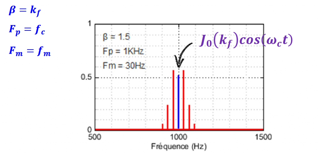
We get the following answer for our FM signal...
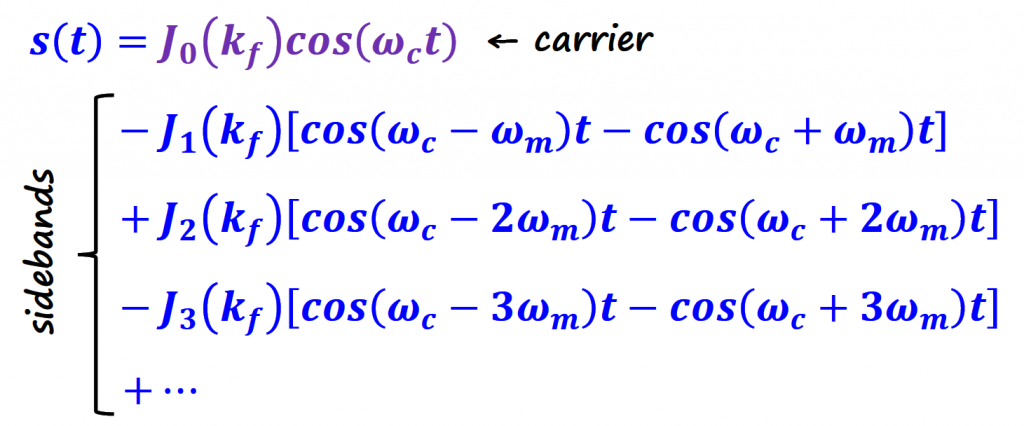
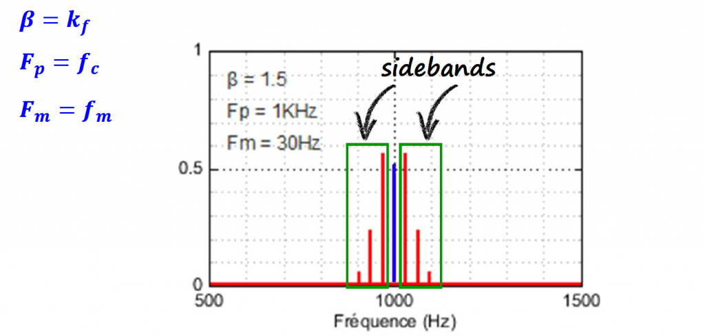
The first term is the carrier, and the rest of the terms are what is called sidebands. If we go to the frequency domain and plot the spectrum of this signal we get the following:
If we plot the spectrum for different scaling factors (kf) we get the following:
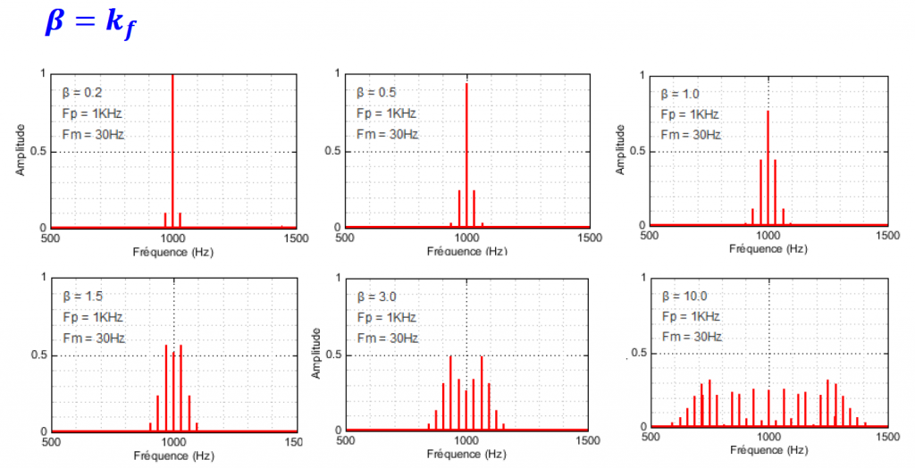
We observe that, has we increase the scaling factor (kf), the power gets distributed amongst the sidebands, and the total power is the same for all graphs.
If we stop here for a moment and think about this, notice that all we are doing by increasing kf is making the Bessel functions give values that are closer to each other. The animation below shows a green line moving around, representing that kf changing over time.
That means that the sinusoidal functions that use those Bessel functions as coefficients, get more equal to each other but at different frequencies. In turn that translates to a wider spectrum.
Wolfram Website has a demonstration that illustrates the power content of FM and PM using one sinusoidal tone as the modulating signal.
On the example above, I am changing only one variable, the scaling factor (k = kf), and we can observe the number of sidebands changing accordingly.
I think it is also cool to see the time domain signal of the resulting FM modulation. Plugging in all the required equations on Desmos, we get the following result:
In this particular example, I am plotting in green an FM modulated signal with kf = 4, and in red an FM modulated signal with kf = 2. Then I am varying the information signal (m(t)) frequency between a range of values back and forth.
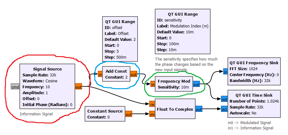
Finally lets implement a simple FM modulator using GNURadio.
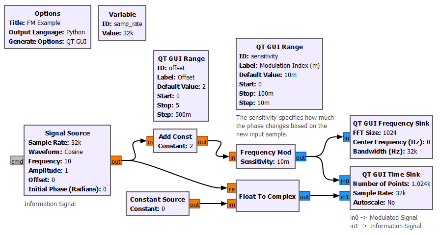
As we increase the modulation index, we can see in the spectrum the number of sidebands increasing.
NFM vs WFM
After plotting and having fun with different values of the scaling factor (kf), the question that we might ask at this point is, which kf should I use in my applications ?
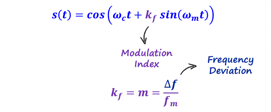
The scaling factor is also called modulation index (m), and m determines the occupied bandwidth. It is a measure of the bandwidth of the signal by taking the ratio between frequency deviation and the maximum frequency (fm) of the information signal (m(t)).
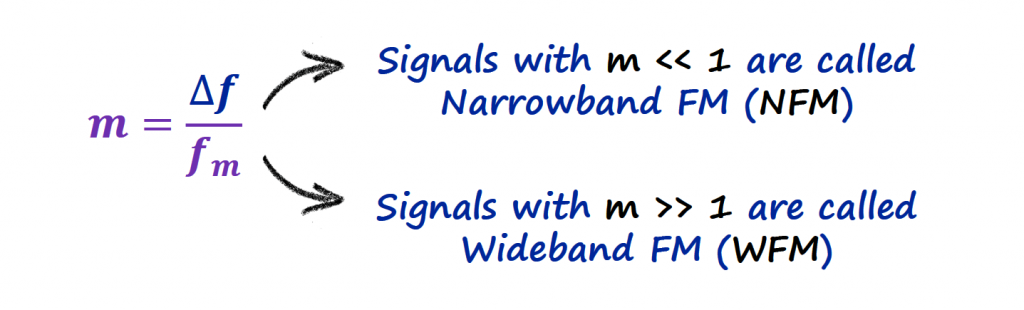
If m << 1 then we are dealing with a Narrowband FM (NFM) modulation, and if m >> 1 then we have a Wideband FM (WFM) modulation.
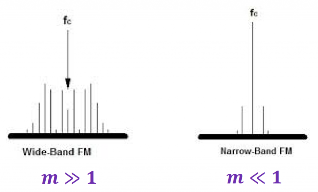
With this information, if we go to the frequency domain and look at how the sidebands are spread across the spectrum, we can get an educated guess on what type of FM modulation is being used.
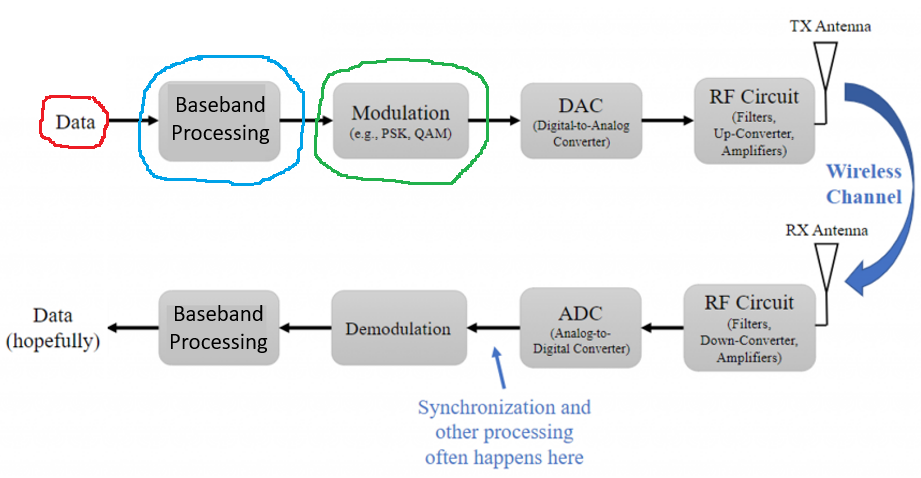
GNURadio Flowgraph <=> Tx-Rx Chain Block Diagram
We implemented the FM scheme with GNURadio flowgraph, and this section goal is to relate this flowgraph with the Tx-Rx Chain block diagram introduced in the Intro section of the Analog Data to Analog Signal topic.
Modulation
GNURadio Files
- Frequency Direction Example
- FM Modulation Example
References
- [Ref 1] “PySDR: A Guide to SDR and DSP using Python”, PySDR Website [Articles]
- [Ref 2] “Tutorial 17: Frequency Modulation (FM), FSK, MSK and more”, Complex to Real Website, Charan Langton [Article]
- [Ref 3] “Tutorials on Digital Communications”, Complex to Real Website, Charan Langton
- [Ref 4] “Summary of Trigonometric Identities”, Clark University [Article]
- [Ref 5] “Modern Digital and Analog Communication Systems”, B. P. Lathi and Zhi Ding [Book]