Fundamental Knowledge
The goal with this section is to introduce the reader to fundamental knowledge and language that will help to understand better the building blocks presented in future articles.
Information vs Communication Theory
It is very easy to get lost and confused when studying concepts for digital communications. One of the main reasons is the interception of different fields of study, such as Information Theory, Communication Theory, and Signal Processing.
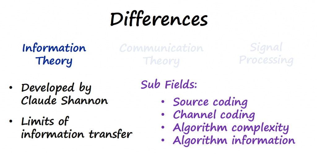
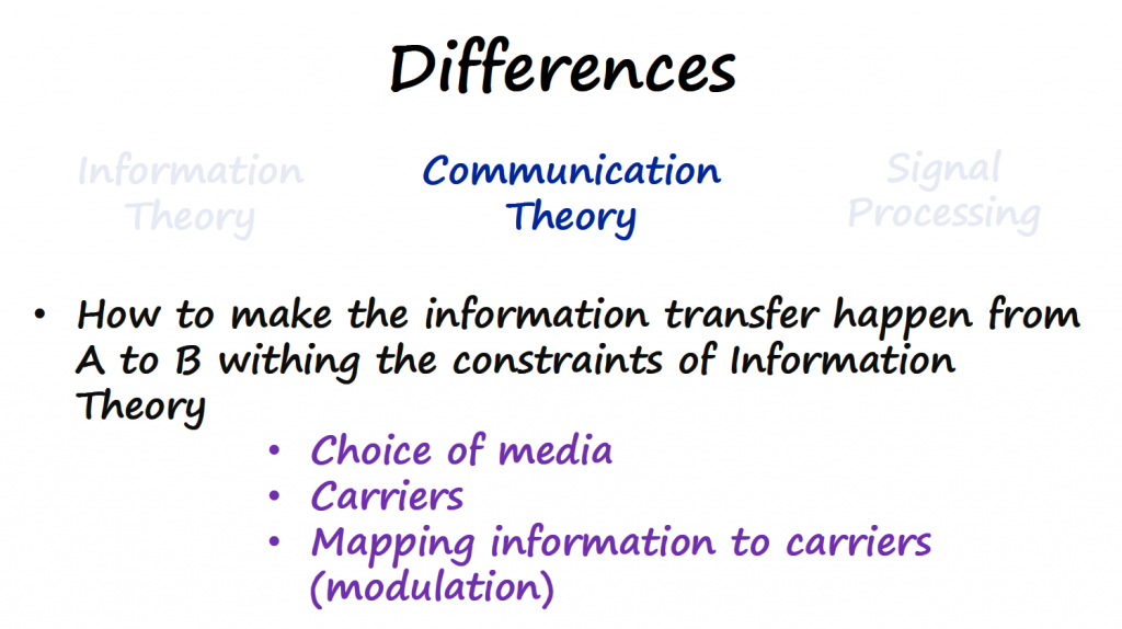
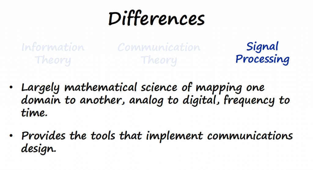
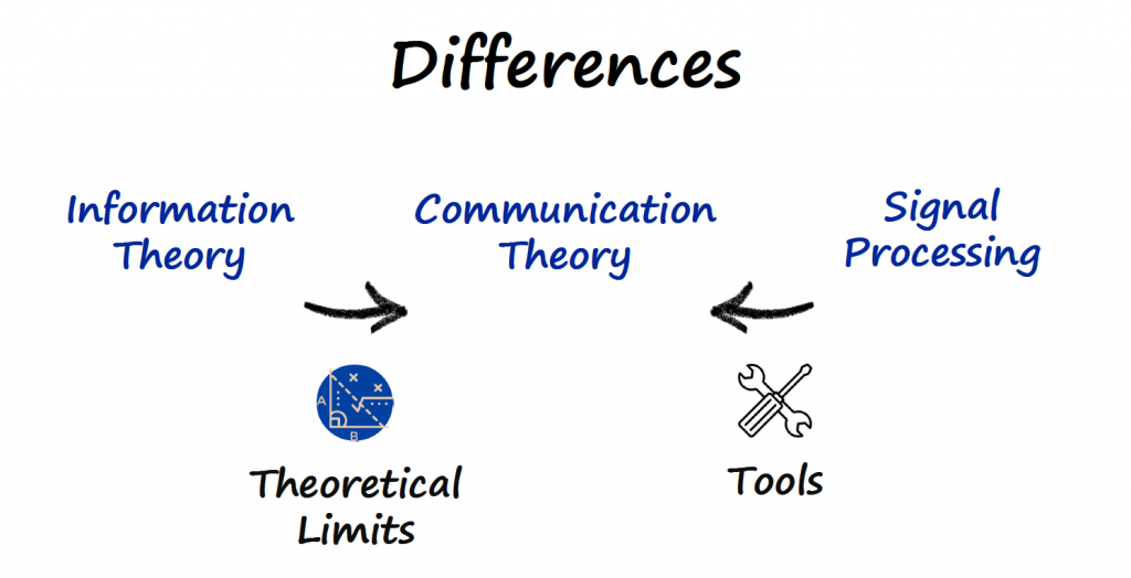
Any digital communication project can contain concepts from these 3 fields at the same time, and not knowing or not being aware of the different concepts covered by each field can make the study of digital communications more difficult.
Tx-Rx Chain Block Diagram
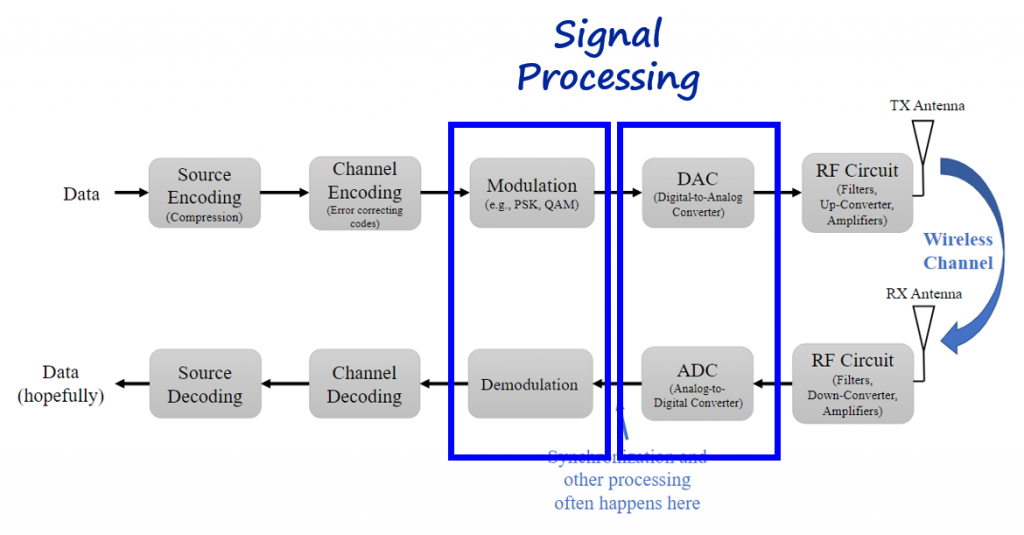
Since we are dealing with SDRs to transmit information between a transmitter and a receiver, another way to organize the concepts presented on the previous section is by using the Transmit-Receive or Tx-Rx Chain block diagram below.
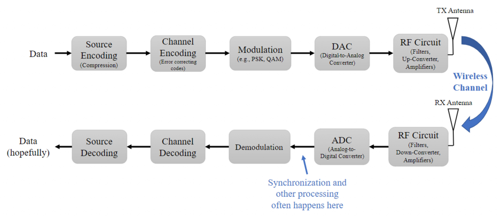
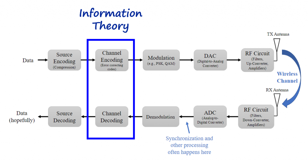
Information theory concepts are normally present on the channel encoding and decoding modules.
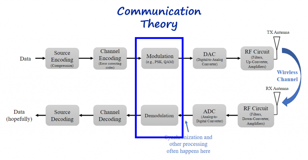
Communication theory concepts are present on the modulation and demodulation modules.
And signal processing concepts (mainly filters and sampling rates adjustments) are present at the modulation, demodulation, DAC and ADC modules.
Modulation Schemes
There are 3 types of signals in digital communications: information signal, carrier and modulated signal. The relationship between these 3 types of signal is the following:
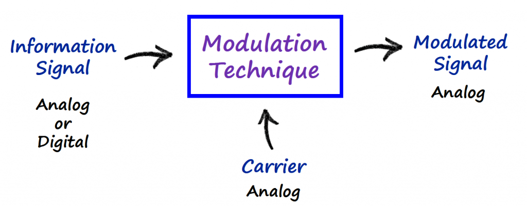
- Information signal (or baseband signals): is the information that we want to communicate. These are signals that contain information either in analog or digital form. Normally these signals are less than 50 kHz (voice, music, video, and data).
- Carrier: carries the information signal over long distances. It is a pure sinusoid of a particular frequency and phase. The frequency of a carrier is usually much higher than the information signal. The choice of a carrier is a function of the medium it must pass through.
- For wired comms around kHz range
- For wireless comms between MHz and GHz range
- The following chart (Link) shows the allocation and regulation of the electromagnetic spectrum into radio frequency bands, normally done by governments in most countries.
- Modulated signal: is a carrier that has been loaded with an information signal.
- Modulation: is the process of taking either an analog or a digital signal and turning it into an analog signal.
There are 4 different types of modulation techniques.
Analog Data to Analog Signal
Analog Data to Digital Signal
Pulse Modulation
- Analog
- Pulse Amplitude Modulation (PAM)
- Pulse Width Modulation (PWM)
- Pulse Position Modulation (PPM)
- Digital
- Pulse-Code Modulation (PCM)
- Differential PCM (DPCM)
- Adaptive DPCM (ADPCM)
- Delta Modulation (DM or Δ-Modulation)
- Delta-Sigma Modulation (ΣΔ)
- Adaptive-Delta (ADM)
- Pulse Density (PDM)
- Pulse-Code Modulation (PCM)
Digital Data to Analog Signal
Passband
- Amplitude Shift Keying (ASK)
- On-Off Keying (OOK)
- M-ary ASK
- Frequency Shift Keying (FSK)
- Audio FSK (AFSK)
- Multi Frequency (M-ary FSK)
- Dual-Tone Multi Frequency (DTMF)
- Phase Shift Keying (PSK)
- Binary PSK (BPSK)
- Quadrature PSK (QPSK, 8PSK, 16PSK)
- Differential PSK (DPSK)
- Offset QPSK (OQPSK)
- π/4-QPSK
- Quadrature AM (QAM)
- Continuous Phase Modulation
- Minimum Shift Keying (MSK)
- Gaussian MSK (GMSK)
- Continuous Phase FSK (CPFSK)
- Orthogonal FDM (OFDM)
- Discrete Multi Tone (DMT)
- Wavelet Modulation
- Trellis Coded Modulation (TCM)
- Spread-Spectrum Techniques
- Direct-Sequence SS (DSSS)
- Chirp SS (CSS)
- Frequency-Hopping SS (FHSS)
Digital Data to Digital Signal
Baseband
- Non Return to Zero (NRZ)
- NRZ Inverted (NRZI)
- Manchester
- Bipolar Encoding
Frequency Domain
[Ref 1] does a very good job introducing frequency domain concepts and covers Fourier Series, Fourier Transform, Fourier properties, FFT, windowing, and spectrograms. If you are not familiar with these concepts or need a refresher, go ahead and read that reference first before continuing.
Let's start using GNURadio to implement some of the Time-Frequency properties that are present on SDRs, and get an understanding on what those properties do to signals in the respective domain.
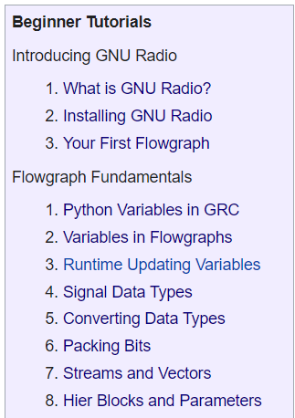
Note: if this is the first time that you are encountering GNURadio concepts, I recommend going over the Introduction and Flowgraph Fundamentals from the Beginners tutorial first.
Linearity Property
If we add two signals in time, then the frequency domain version will also be the two frequency domain signals added together.
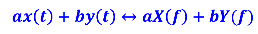
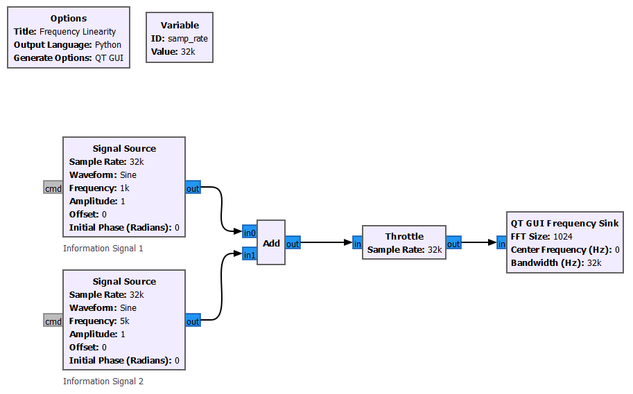
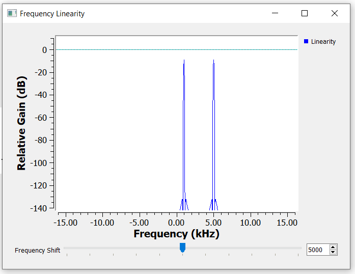
This property is useful when for example we need to add voice and video together on the same communication channel. Adding the signals in time, will add the respective spectrum in the frequency domain. In this simple example, we are adding two sinusoidal waves at different frequencies but we need extra care if the spectrum of the two signals of interest overlap.
Frequency Shift Property
If you remember on the previous section, a modulated signal is a carrier that has been loaded with an information signal.
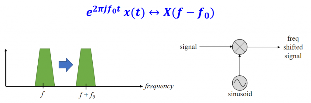
The most basic way to modulate a signal is to multiply the information signal with the carrier. Since we are multiplying a signal with a pure sinusoidal waveform (carrier) in time, that corresponds to shift that same signal by the carrier frequency in the frequency domain.
Below you can see this concept represented in different ways. In blue you have the mathematical description of this operation in time and respective frequency domain; the graph with green shapes shows the frequency domain result of the shift operation; and the block diagram on the right represents the mathematical operation done in the time domain (the multiplication of the signal with the carrier).
With GNURadio we can build the blocks similar to the time domain block diagram on the right and then use graphic analyzers to view the signal in time and/or frequency domain.
For simplicity, the building blocks below, start by multiplying one sinusoidal waveform at 1kHz as the information signal with a carrier at 5 kHz.
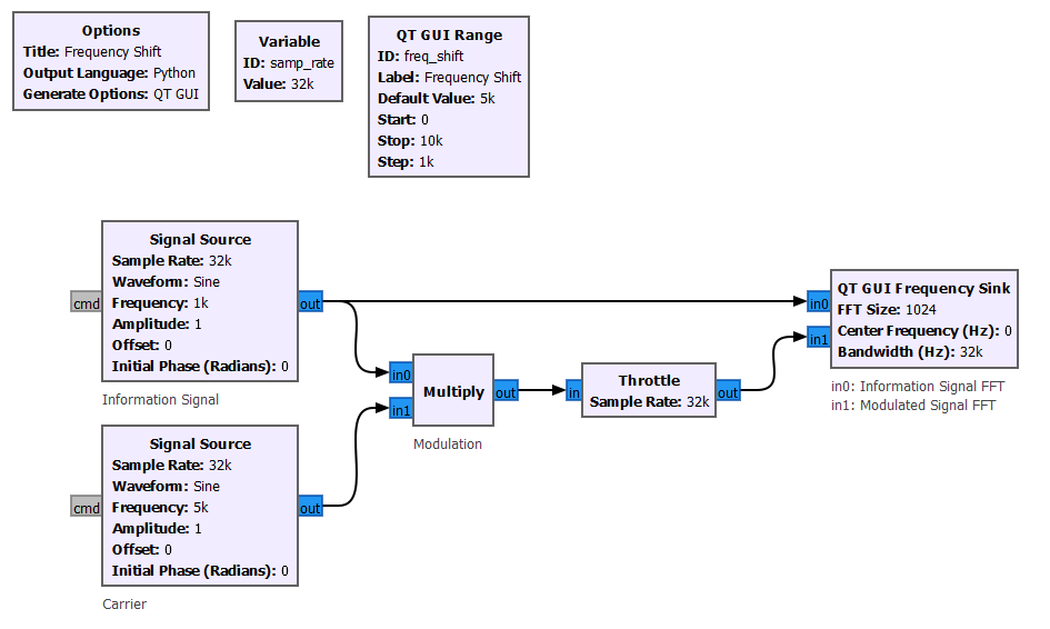
I am using a Frequency Sink block to check the result in the frequency domain. Notice on how the shifted signal (in red - Plot 1) is the original signal (in blue - Plot 1) shifted by the frequency of the carrier in the frequency domain.
Information signals are going to be more complex than just a simple sinusoidal waveform. The figure below shows another example, by using a triangle waveform as the information signal.
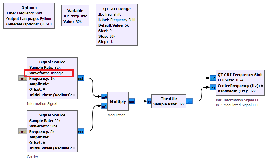
As expected, a triangle waveform as more spectral content than a single sinusoidal waveform. Notice on how all the components of the spectrum shift equally when we change the carrier frequency.
Scaling in Time Property
Scaling in time essentially shrinks or expands the signal in the x-axis. When we transmit bits faster we have to use more frequencies.
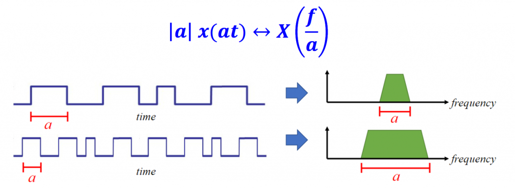
This property helps to explain why higher data rate signals take up more bandwidth/spectrum.
Convolution in Time Property
It is called convolution property because in the time domain we are convolving x(t) with y(t). However, in the frequency domain that is equivalent to multiplying the frequency domain versions of those two signals.
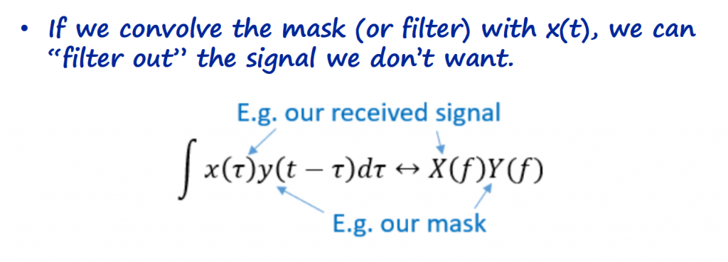
Convolution is widely applied in the time domain when filters are used in the frequency domain to remove unwanted signals from the spectrum.
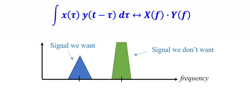
Normally, y(t) is the mask (or filter) we want to apply in the frequency domain.
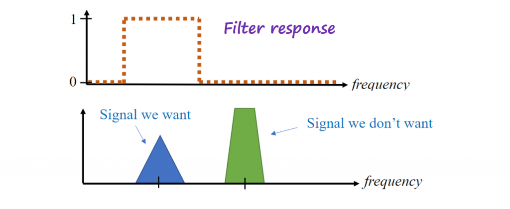
Perfect filters have a rectangular shape in the frequency domain, which corresponds to a sinc function (y(t)) in the time domain. The sinc pulse continues to both positive and negative infinity along the time axis. Whilst mathematically you can readily take the Fourier transform of a sinc pulse, it can’t be computed because of the extension to infinity
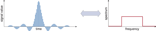
The obvious solution is to truncate the sinc response so that the ripples no longer extend to infinity.
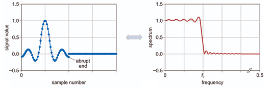
The effects of this in the frequency domain translates to ripples in the passband and the stop band. In essence this shows why you can never have the perfect ideal or ‘brick-wall’ filter.
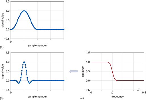
A technique for dealing with the truncated sinc is to apply a window function that brings the endpoints of the truncated sinc to zero.
GNURadio allows you to use FIR (Finite Impulse Response) and IIR (Infinite Impulse Response) digital filters. The difference between these two options is outside the scope of this article.
The example below implements a FIR band pass filter to remove the frequency of the information signal 1 (@1kHz).
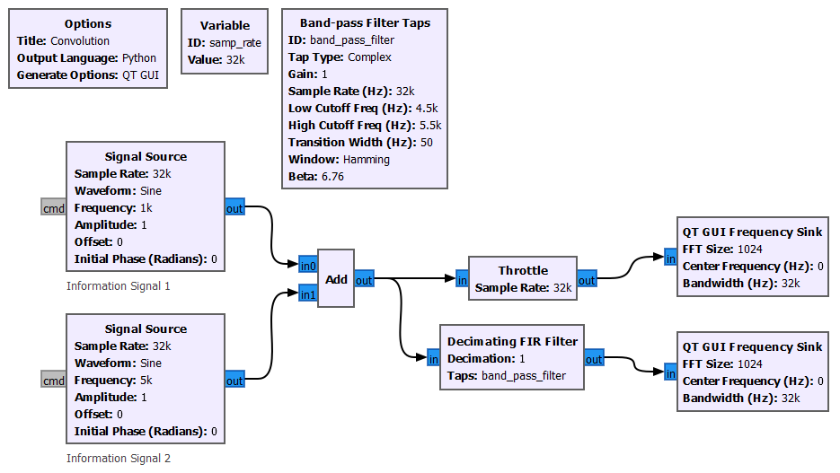
The "Decimation FIR Filter" block uses the fir_filter_XXX function (Link) that creates a finite impulse response (FIR) filter that performs the convolution in the time domain. There are a couple of different ways to define and create filters specs (or taps) with GNURadio, but for now we are using the "Band-pass Filter Taps" block that creates the desired specs in a more user friendly way.
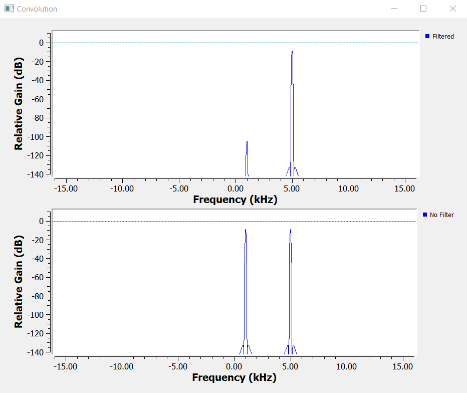
The result after applying the band pass filter around information signal 2 (@ 5kHz), is the considerable reduction of the information signal 1 amplitude (@ 1kHz).
IQ Sampling
IQ sampling is another core concept into understanding SDRs, and it can also be very confusing while studying it for the first time. The main reason is because there is a lot of math (e.g.: basis functions, orthogonal sets, complex numbers, exponential Fourier series, Euler's identity, trigonometric identities, etc) involved to explain and validate this concept, but besides all that math it is in fact very simple to use and implement it.
Complex Numbers
In essence we are representing the information signal as a complex number (we will see later how that conversion/representation is done), that contains a real and imaginary part. We can write those complex numbers in the complex plane (or Argand diagram) as a cartesian coordinate (z = a + bi) or as polar coordinate (z = r ∟ϕ).
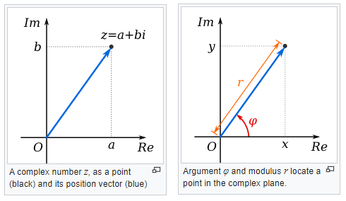
Notice on how we can represent this complex number as vector too, with a direction and magnitude.
There is one more concept that we need to introduce in order to close the loop on understanding IQ sampling, and that is the Euler Formula...
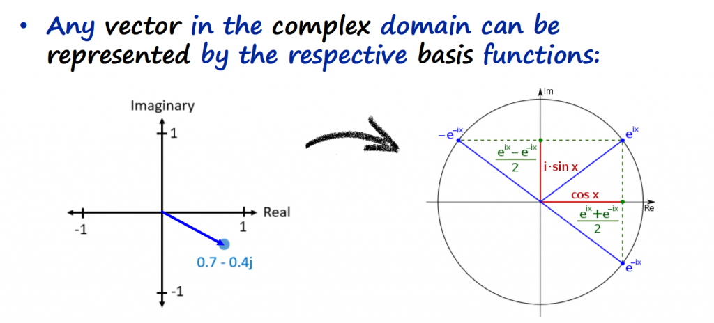
Remember that basis functions in this context, are vectors that are orthogonal to each other. If vectors are orthogonal to each other, they can happen at the same time (they don't overlap).
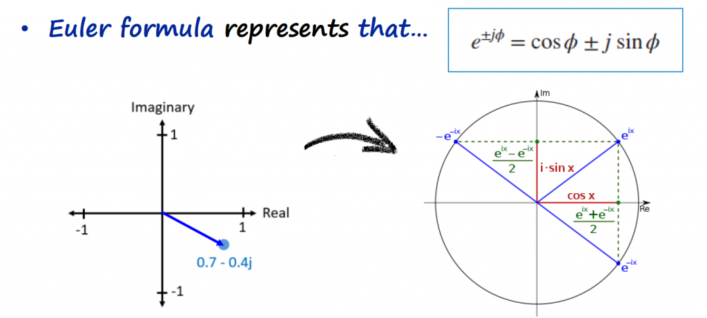
Euler formula is just telling us that any complex vector is a combination of a cosine and sine basis function, orthogonal to each other. For now, we are going to accept this, and I will leave the explanation on how to get to the Euler formula this article (Link).
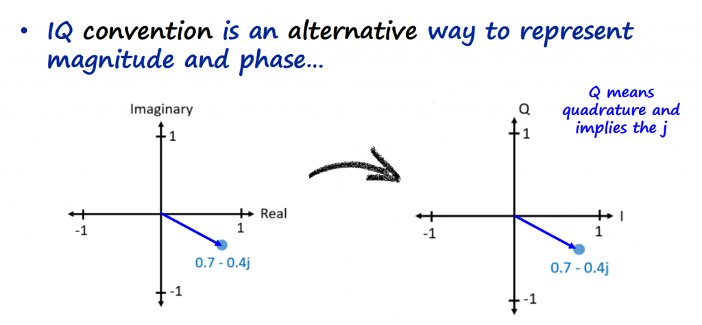
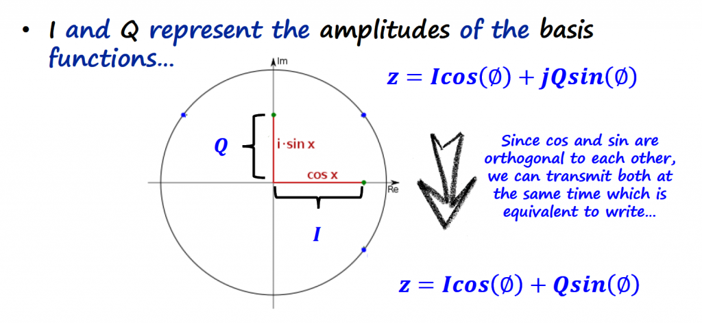
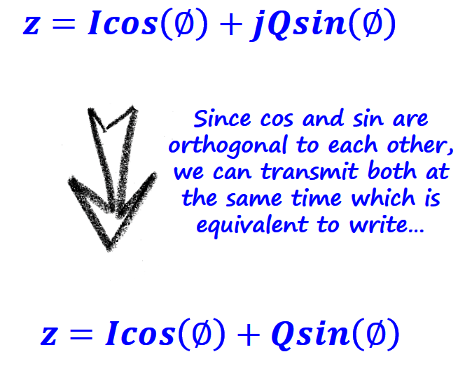
If we combine the IQ convention with the Euler's formula we get the following:
IQ Channels
The term "quadrature" has many meanings, but in the context of DSP an SDR it refers to two waves that are 90 degrees out of phase (orthogonal to each other).
In the previous section we saw that the IQ representation of a complex number is:
You can play with the Desmos animation below and check it for yourself.
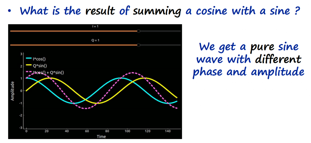
The beauty of this IQ channel concept, is that it is very easy to control the amplitude and phase of the resultant sinusoidal waveform just by controlling two gains, I an Q.
Have in mind...
We often talk about complex and real signals in communications, but all physical signals are real. Complexness of signals is a mathematical construct that is used with information signals (or baseband) processing.
IQ Transmitter
Let's go over on how to transmit IQ data, and let's assume that we want to transmit the complex number 0.7 - 0.4j or the respective IQ value 0.7cos(θ) - 0.4sin(θ)
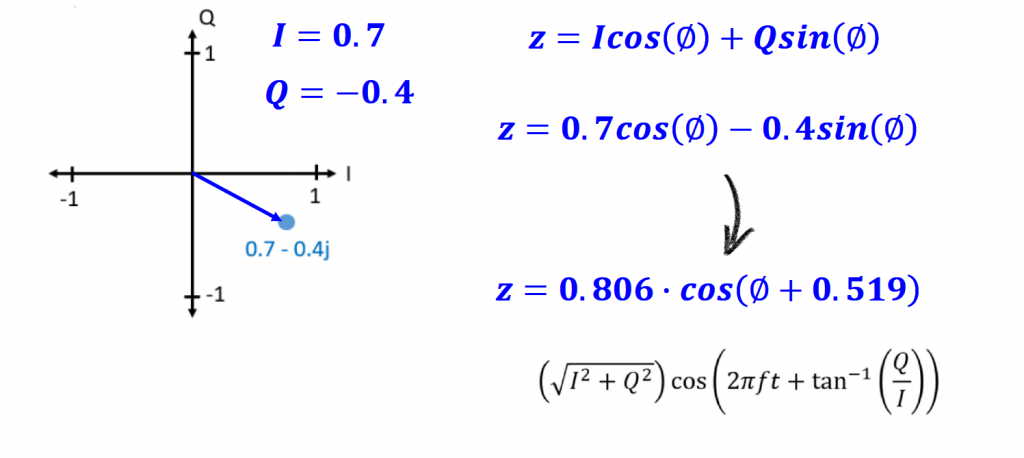
In terms of block diagram, we need to feed the I and Q values to the respective multiplication block. We only need to have one sinusoidal waveform (cosine) and shift it by 90 degrees to obtain the orthogonal signal.
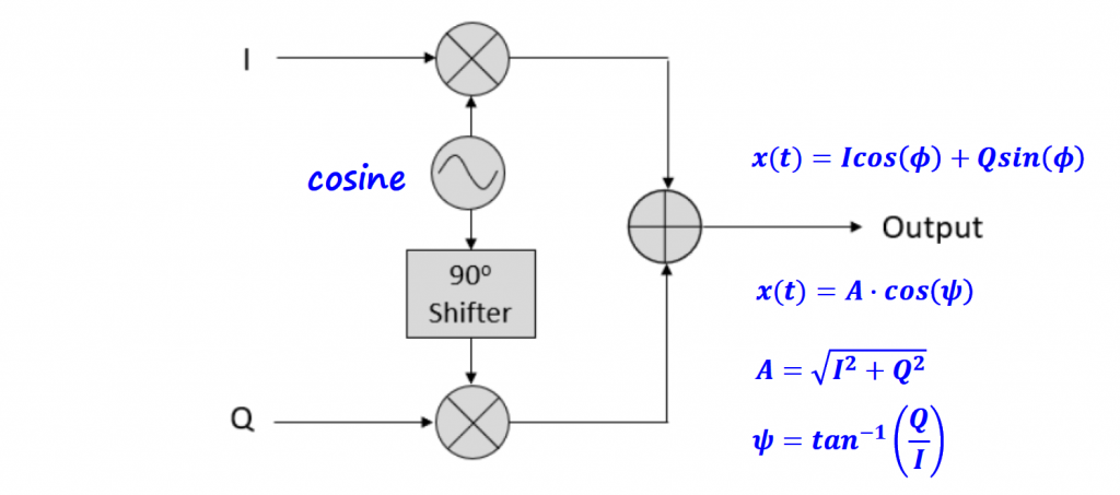
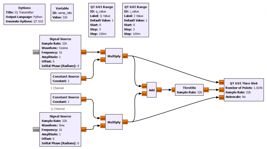
In terms of GNURadio building blocks, the block diagram below shows the simple concept of an IQ transmitter.
IQ Receiver
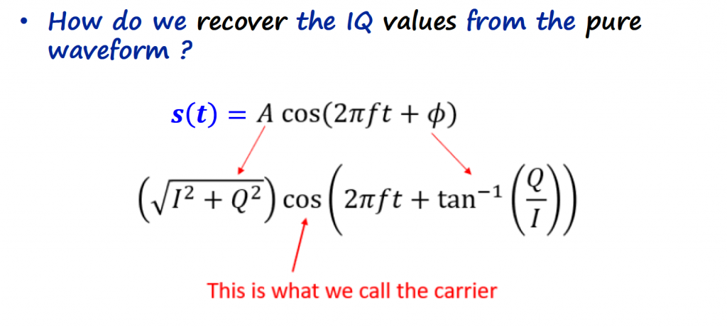
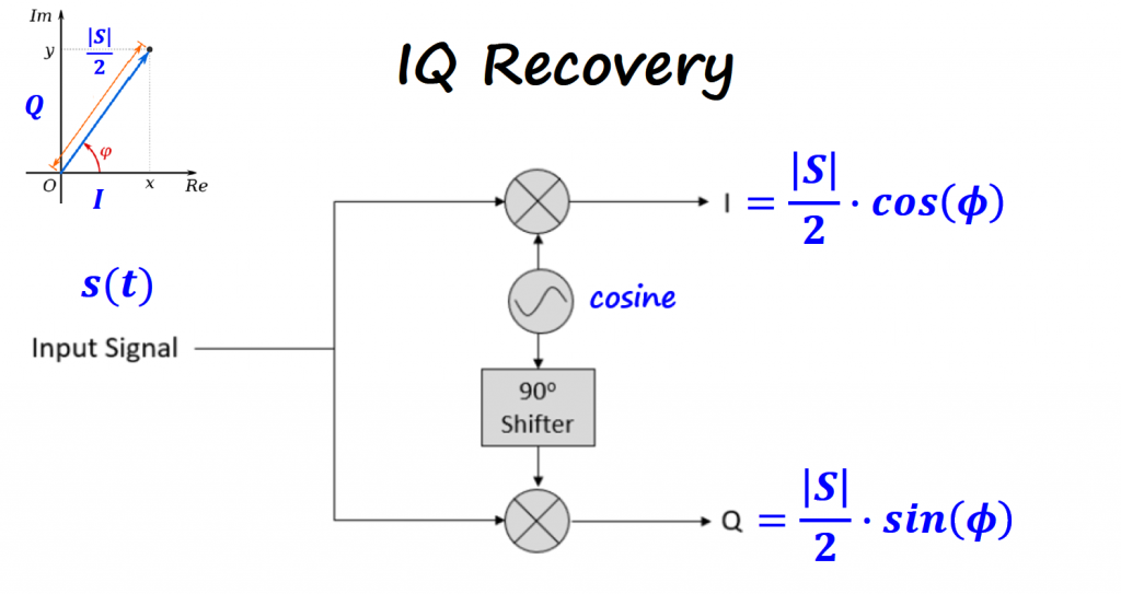
The simplest IQ recovery system relies on multiplying the received signal with the basis functions used to created the IQ signal.
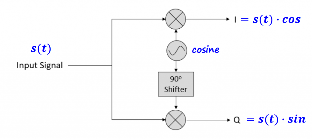
At the end we have the IQ recovery system below. The angle θ is not that simple as depicted in the system, but for simplicity we keep it like that for now.
IQ Plots/Constellations
When we start modulating the information signal with IQ values, the time and frequency domain visualizations make it hard to visualize what is going on during communications.
IQ plots make a better tool to visualize the contents that are being transmitted and received.
Remember that...
That is what IQ plots are, a way to represent IQ values.
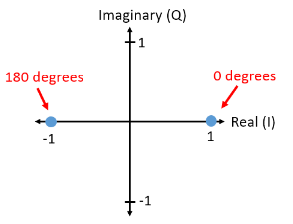
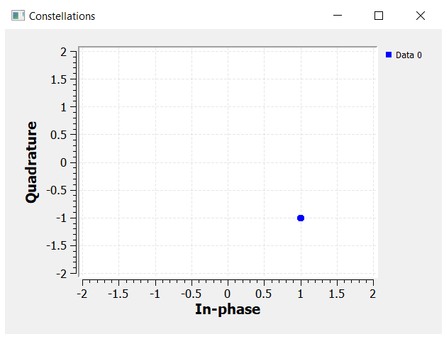
When the IQ plots start representing information being transmitted, the points on those plots form patterns that are called constellations. Constellations can have different shapes depending on the type of modulation scheme and it can become quite busy...
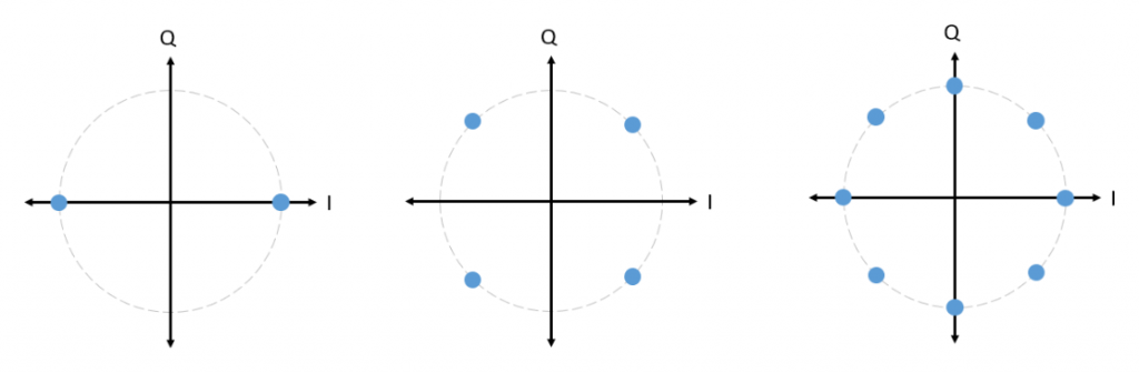
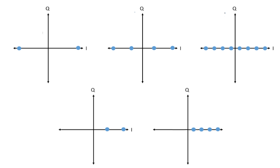
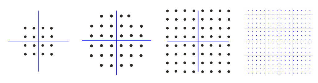
Each dot on the constellation is an IQ value, and we will see later on how to related the information signal to an IQ value.
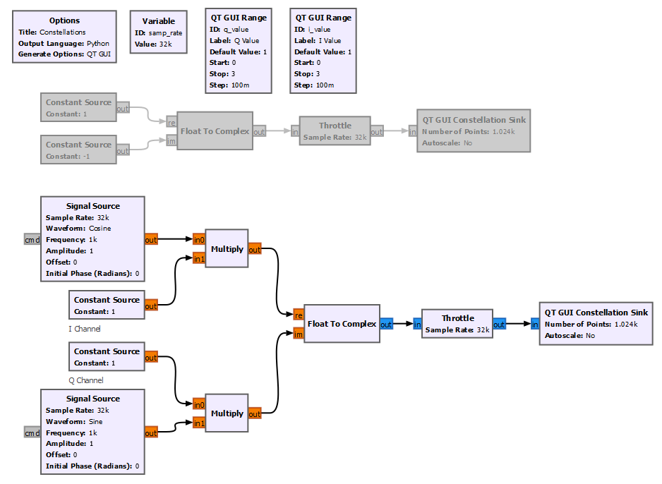
To visualize constellations in GNURadio, we can use the block "QT GUI Constellations Sink". The example below, plots the IQ value 1 - 1j (4th quadrant).
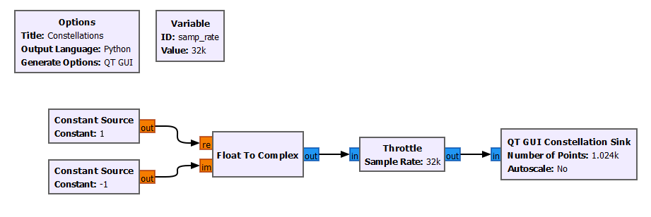
We can also add the constellation sink block to the IQ transmitter block diagram presented on the previous section and observe how the IQ values get mapped into the constellation map.
By manipulating I and Q, we can set the magnitude of the Euler's identity components accordingly. We can have pure real numbers by setting Q = 0, and pure imaginary numbers by setting I = 0.
GNURadio Files
- Frequency Linearity Example
- Frequency Shift Example
- Convolution Example
- IQ Transmitter Example
- IQ Plots/Constellations Example
References
- [Ref 1] “PySDR: A Guide to SDR and DSP using Python”, PySDR Website [Articles]
- [Ref 2] “Tutorial 1: Basic concepts in signal analysis, power, energy and spectrum”, Complex to Real Website, Charan Langton [Article]
- [Ref 3] “Fourier transforms and the sinc pulse”, Open Learn [Article]
- [Ref 4] “Tutorial 8: All About Modulation”, Complex to Real Website, Charan Langton [Article]
- [Ref 5] “Tutorials on Digital Communications”, Complex to Real Website, Charan Langton
- [Ref 6] “Summary of Trigonometric Identities”, Clark University [Article]