NI Acquisition Strategies
On articles related with NI-DAQs and python code, you can see different ways to interact with the DAQ when acquiring analog samples. You will see the use of either QTimers or Threads or NI callback functions.
Note: quick note about the use of the word DAQ throughout this article: DAQ stands for Digital AcQuisition board and it is the instrument used to translate sensor and signal data into a digital format that is sent to a computer to process that data. DAQs have ADCs (Analog to Digital Converters) that are responsible to convert analog to digital signals, and/or DACs (Digital to Analog Converters) that are used to generate analog signals. The concepts of this article are related mainly with the ADC part of the DAQ, but I am going to use the word DAQ since the concepts are more in scope with on how the software interacts with the DAQ than the ADC.
The reader with no experience in programming might get confused reading those articles, and can question what and when to use QTimers, Threads or callback functions. The goal with this article is to hopefully clarify some of these approaches and understand which one is more suitable for your application.
Remember that are pros and cons with any approach, and the way to go is to understand what each technique has to offer and select the one that works best with your application requirements and constraints.
I am going to focus on the acquisition of analog samples, since that is the one that can be the most confusing to set up properly. However, the techniques explained here can be applied in a similar way if your analog outputs or digital inputs/outputs need to be done in a determinist way.
Nyquist and Sampling Rate
When dealing with analog samples, we need to be aware of the sampling rate used to acquire our signals.
Nyquist defines the minimum sampling rate for the highest frequency that you want to measure, to be x2 the given frequency to be measured accurately. For example, if in your application you know that the maximum frequency that you will get is 1kHz, then you should at least sample 2 times that speed (2kHz).
We can visualize this statement in two different ways: in time and in frequency domain. If you are not familiar with time and frequency domains, check out [REF 2], it will give you a quick overview with all the necessary information to follow along this article.
[REF 1] is another reference that does a fantastic job showing why we need to sample twice of the highest frequency that you want to measure in the time domain.
And finally, the Aliasing Wikipedia article has an animated picture that glues all these views and concepts together.
- The first column of graphs are time domain views and the second column of graphs are the frequency domain view.
- For the first row, the time domain view is rendering the analog input (continuous blue line) and the sampled values (blue dots). The graph sweeps the analog input from 0*fs to 1*fs in increments of 0.01.
- Notice that the blue dots can pretty much fit on the analog input until around 0.5*fs (also called the Nyquist frequency). After that the blue dots are all over the place on the analog input.
- The reconstruction of the available samples is shown on the second row in orange, and we can see that until the analog input frequency exceeds the Nyquist frequency, the reconstruction matches the actual waveform. After that, it is the low frequency alias of the analog input.
- The frequency of that reconstructed signal after the Nyquist frequency is also called folding frequency.
Let's Observe Aliasing
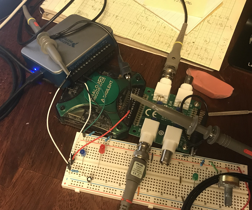
Before writing any code, let's observe aliasing in a lab bench setup.
I am going to use two different DAQs that are going to work at different sampling rates so we can observe and compare results accordingly.
- The first DAQ is the Analog Discovery 2 from Digilent that has a maximum sampling rate of 30MHz. According to Nyquist we should be able to get good samples signal reconstruction up to an analog input of 15MHz.
- This DAQ adjusts the sampling rate automatically as you adjust the time base of the oscilloscope, so I can't use this DAQ alone to show the aliasing effect.
- However, the waveforms software that is available to interact with this DAQ can show the frequency domain in real time.
- I am going to use this DAQ to show the frequency domain and as a function generator.
- The second DAQ is the NI USB-6002 that has a maximum sampling rate of 50kHz. According to Nyquist we should be able to get good samples signal reconstruction up to an analog input of 25kHz.
- I can change the sampling rate of this DAQ in real time very easily by using the NI-MAX software.
- I am going to use this DAQ to sample the data of the function generator.
Block diagram on how everything is connected
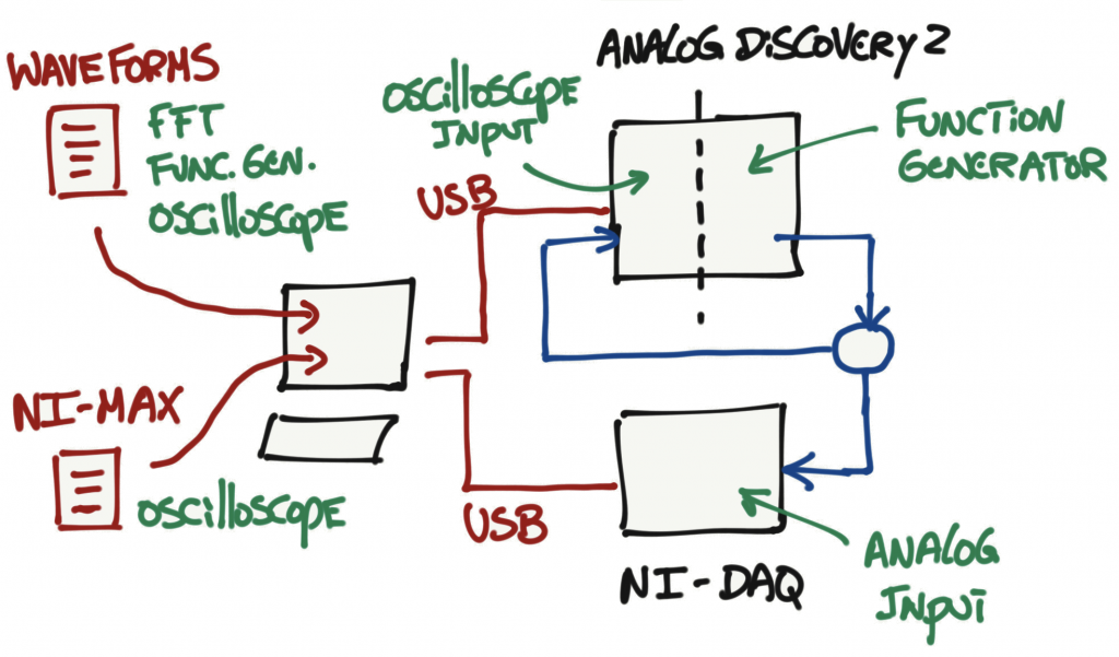
For the tests below, the sampling frequency is going to be fixed to 2kHz, that means that we have a Nyquist frequency of 1kHz. I will vary the analog input frequency (Fin) from 10Hz to 3kHz and observe the aliasing for analog inputs greater than 1kHz.
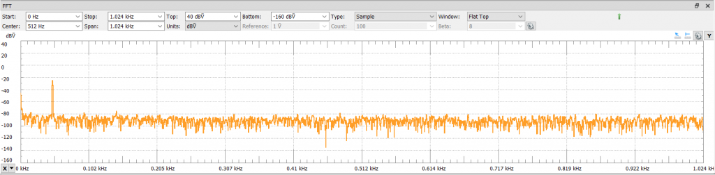
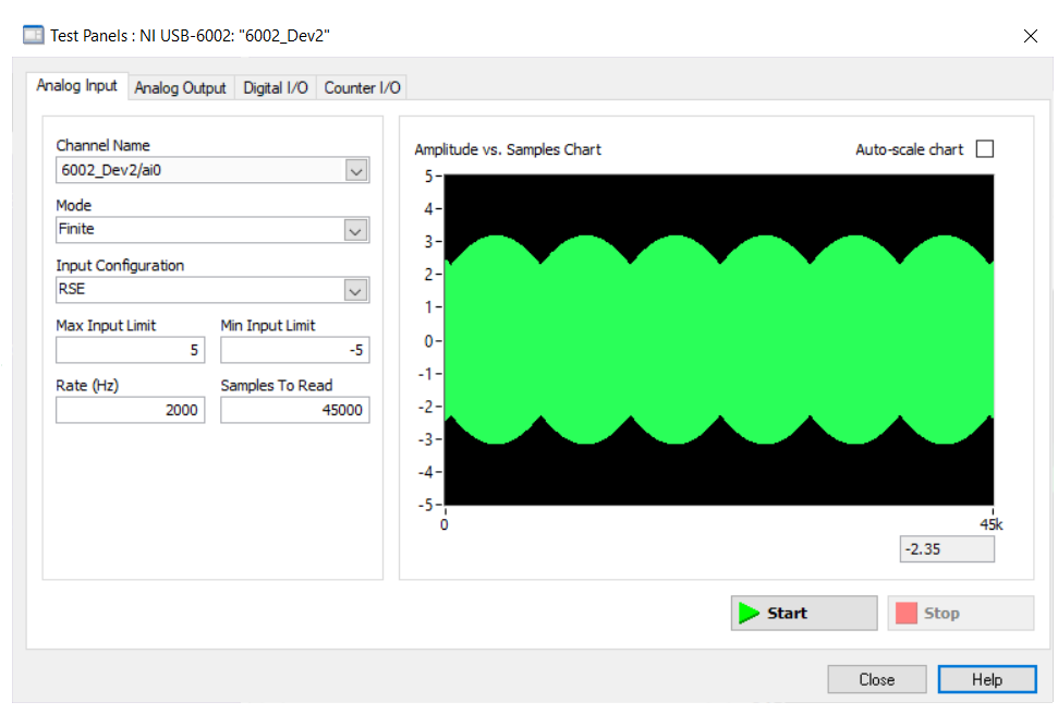
Test 1: Fin = 10Hz
With a sampling rate of 2kHz and an analog input of 10Hz, we should be able to reconstruct the signal with no problem. In this case we have 200 samples available per period to reconstruct the signal. We observe that in the time domain view.
NI-DAQ View - Time Domain

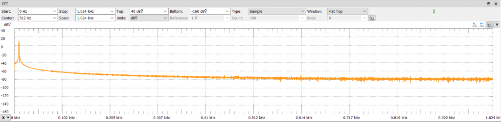
Analog Discovery View - Frequency Domain
In the frequency domain, we have a spike at 10Hz. I want you to notice that I am only showing the spectrum up to the Nyquist frequency so we can observe the aliasing happening later.
Test 2: Fin = 100Hz
With a sampling rate of 2kHz and an analog input of 100Hz, we have 20 samples available per period to reconstruct the signal. Still no problem in the time domain.
NI-DAQ View - Time Domain
Analog Discovery View - Frequency Domain
In the frequency domain we now have a spike at 100Hz.
Test 3: Fin = 200Hz
With a sampling rate of 2kHz and an analog input of 200Hz, we can still reconstruct the signal (10 samples available per period) but you can start seeing some signal degradation in the time domain.
NI-DAQ View - Time Domain
Analog Discovery View - Frequency Domain
In the frequency domain, you have the spike at 200Hz.
Test 4: Fin = 500Hz
With a sampling rate of 2kHz and an analog input of 500Hz, we now have 4 samples available per period and you can see some considerable signal degradation in the time domain. We are half way to the Nyquist frequency and the signal in the time domain is already being affected by the sampling rate.
NI-DAQ View - Time Domain
Analog Discovery View - Frequency Domain
On the other hand, in the frequency domain, all is good. You have a spike at 500Hz.
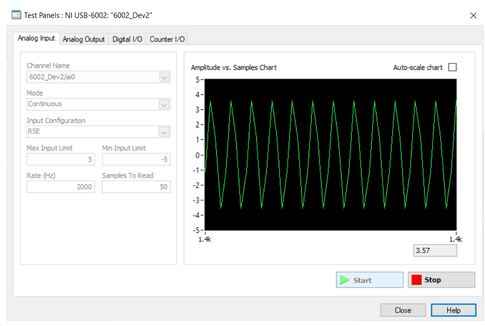
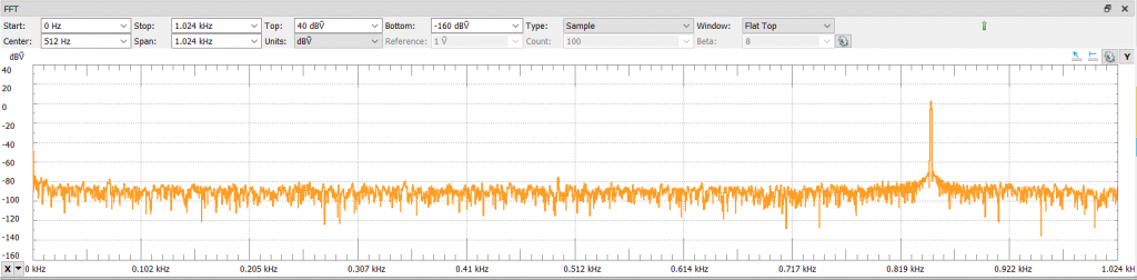
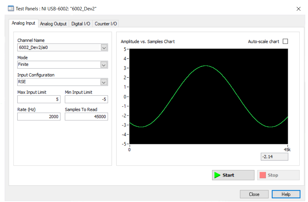
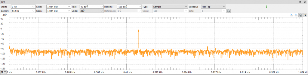
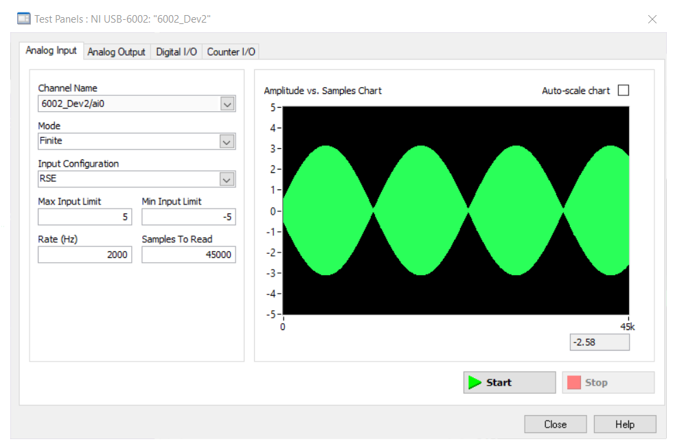
Test 5: Fin = 1kHz
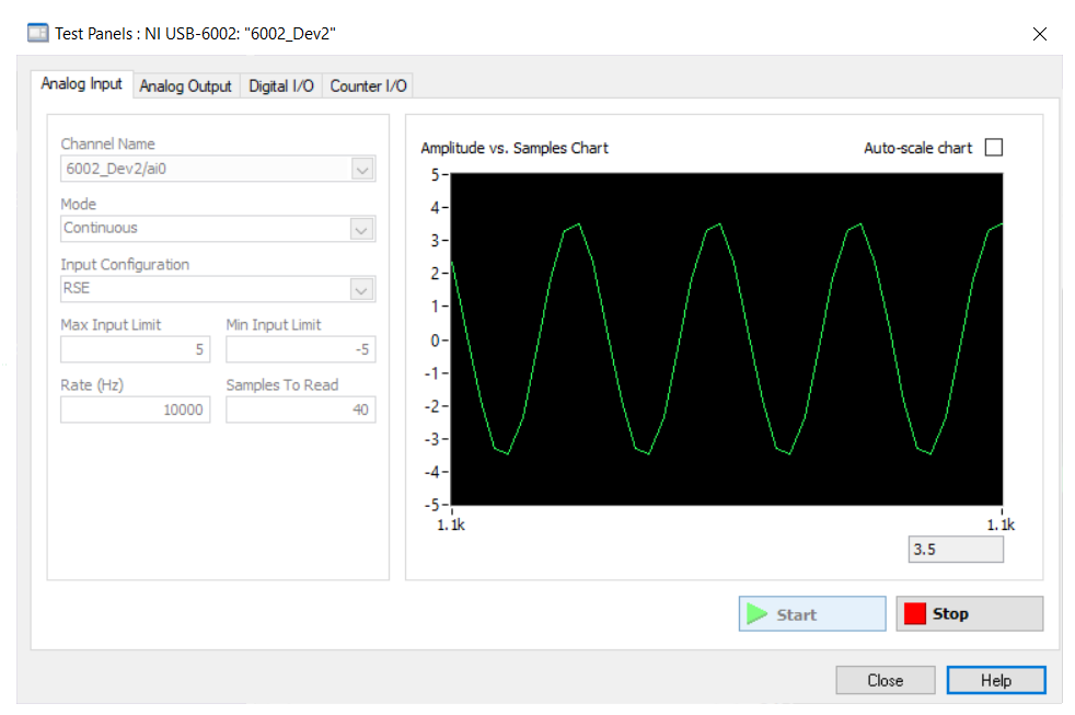
With a sampling rate of 2kHz and an analog input of 1kHz, the signal reconstruction in the time domain gets even worst (2 samples available per period).
NI-DAQ View - Time Domain

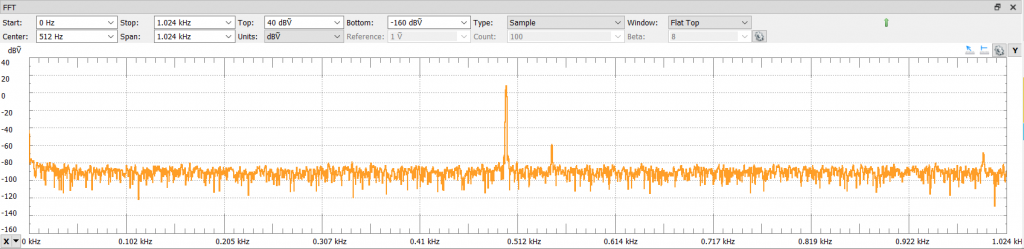
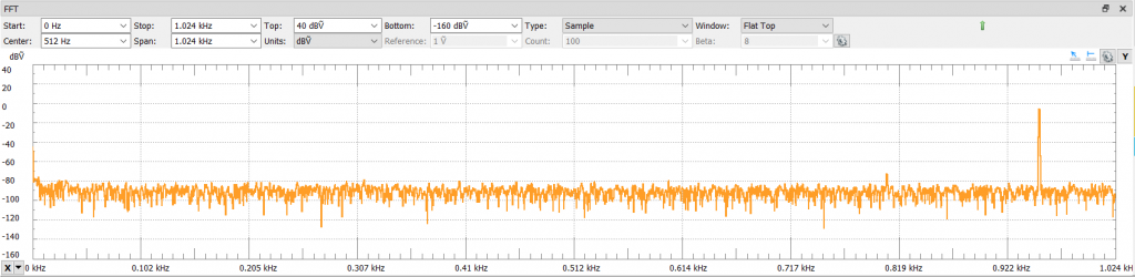
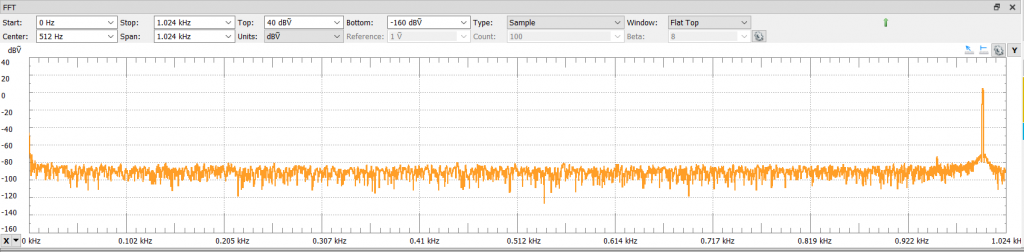
Analog Discovery View - Frequency Domain
In the frequency domain, we still have the spike at the correct frequency.
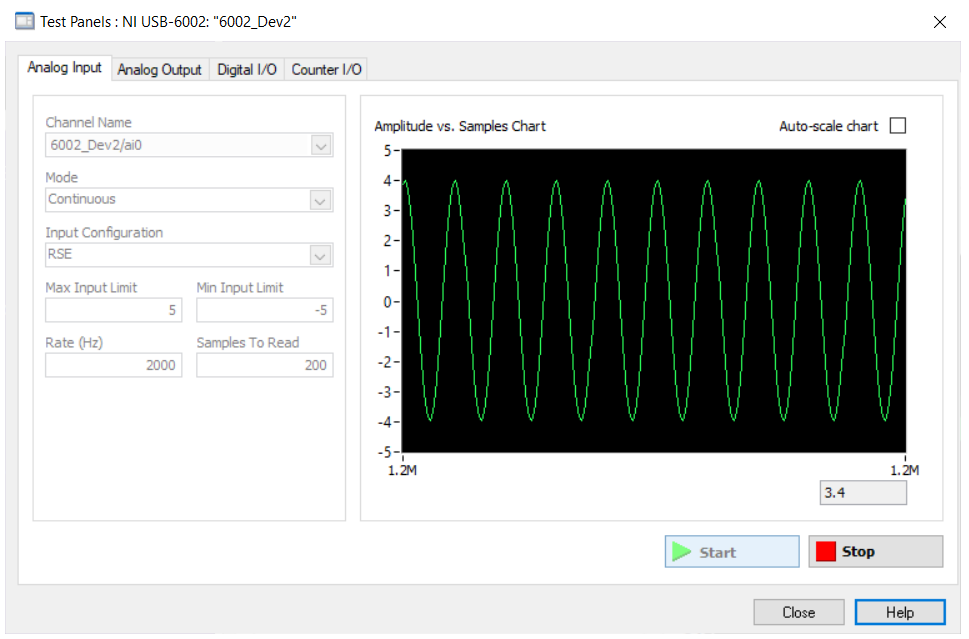
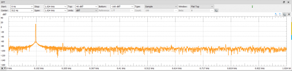
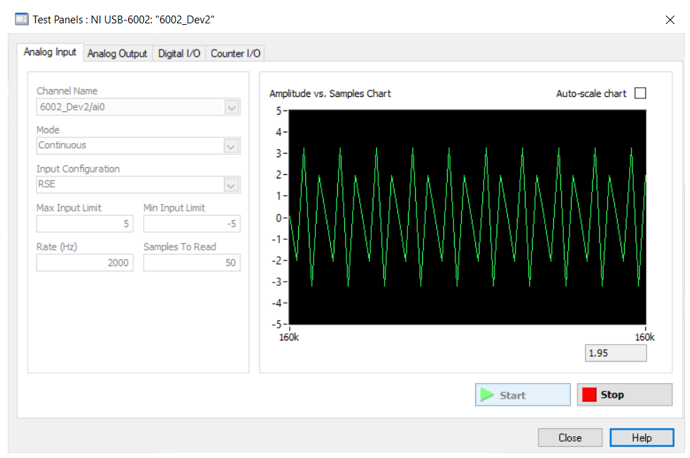
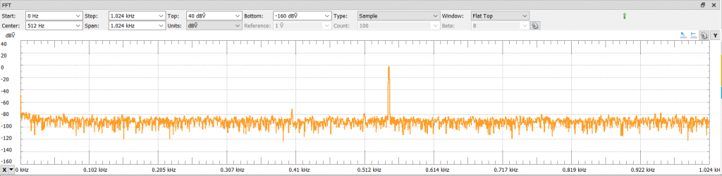
Test 6: Fin = 1.2kHz
Now we start having input signals higher than the Nyquist frequency and we will experience aliasing. With a sampling rate of 2kHz and an analog input of 1.2kHz, the time domain signal is a mess.
NI-DAQ View - Time Domain
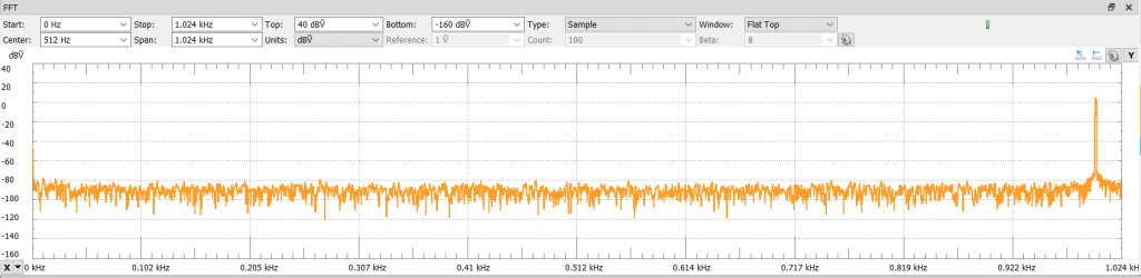
Analog Discovery View - Frequency Domain
In the frequency domain we observe the folding frequency or aliasing of the 1.2kHz signal.
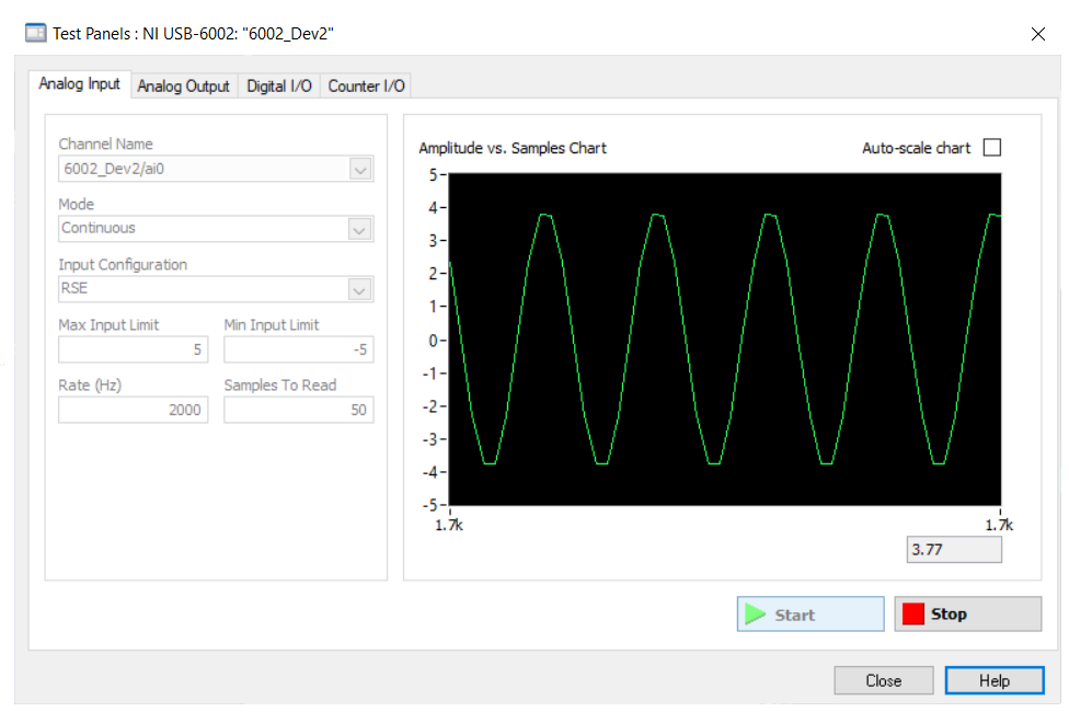
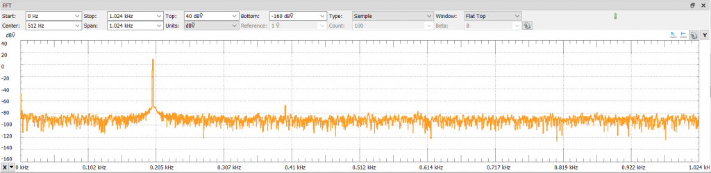
Test 7: Fin = 1.5kHz
With a sampling rate of 2kHz and an analog input of 1.5kHz, we keep having aliasing present in our sampled signal.
NI-DAQ View - Time Domain
Analog Discovery View - Frequency Domain
In the frequency domain you have the respective folding frequency.
Test 8: Fin = 2kHz
With a sampling rate of 2kHz and an analog input of 2kHz, we keep experiencing the folding frequency and in the time domain the reconstructed signal is very low in frequency.
NI-DAQ View - Time Domain
Analog Discovery View - Frequency Domain
Test 9: Fin = 2.5kHz
Passing now the sampling frequency, with a analog input of 2.5kHz, I don't even know how to interpret the time domain signal 😛
NI-DAQ View - Time Domain
Analog Discovery View - Frequency Domain
Aliasing present in the spectrum.
Test 10: Fin = 3kHz
The last one just for fun 🙂
NI-DAQ View - Time Domain
Analog Discovery View - Frequency Domain
Reflections
Hopefully by now you are able to understand the importance of sampling your analog inputs signals with the correct sampling rate and what aliasing is and what looks like in time and frequency domain.
An interesting discovery during the experimentation conducted on the previous section is the fact that complete signal reconstruction in the time domain is good around 10 times less the sampling frequency (good signal up to 200Hz). After that we start seeing some signal degradation in the time domain.
However, in the frequency domain, we are good throughout the all 1kHz of bandwidth.
This is the reason why some resources [REF 4] state the following:
In conclusion, make sure that you know, the best that you can, the signals that are going to be present in your application before choosing the appropriate sampling rate.
- If you are interested in conducting signal analysis in the time domain, you probably need to increase the sampling rate 10 times more instead of 2 times of your Nyquist frequency.
- In our example, with an analog input of 1kHz and increasing the sampling frequency to 10kHz, I can now reconstruct a 1kHz signal in the time domain with no problem.
- If you are interested only in spectra content, 2 or 3 times of your Nyquist frequency is normally sufficient.
Anti-Aliasing Filters
This last section talks about anti-aliasing filters.
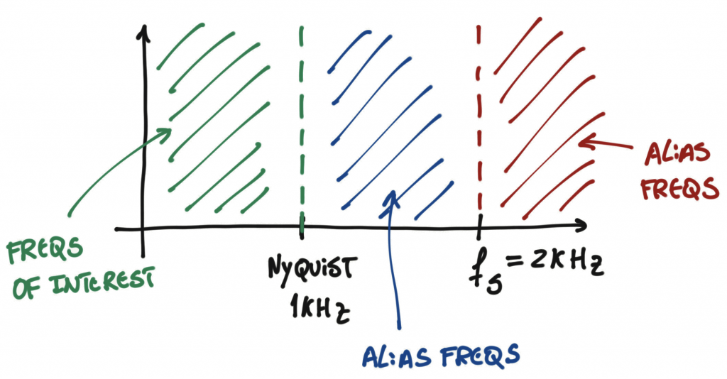
Going back to the example of a sampling rate of 2kHz, and the Nyquist frequency at 1kHz, I will divide the frequency domain into 3 regions.
- The green region, that includes the signals of interest of your application, plus additional alias frequencies if precautions are not taken.
- The blue region, that includes frequencies that are capture with the sampling rate that will show up in the green region as alias frequencies.
- And the red region, that includes frequencies that are not capture by the sampling rate but they will still show up in the green region as alias frequencies.
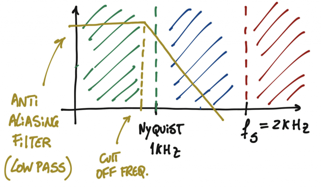
If you experience alias frequencies in your application and that is not a desired effect, you might need to incorporate a low pass filter (also called anti-aliasing filter), in order to eliminate those alias frequencies present in the green region [REF 6].
Have in mind that aliasing is not always bad. For example, in digital communications aliasing can be used to bring signals that are high in frequency to the baseband when you can't sample at fast rates 🙂
If you read the previous sections you know how important it is to sample your signals at the correct sampling rate, otherwise you will get wrong data of your analog input.
When doing the program that will acquire the samples on a normal laptop it can be a challenge to run them at the required sampling rates mainly because you have a lot of programs running in your operating system and your application will most likely not be deterministic.
There are a couple of ways to tackle this problem:
- If you have access to a RTOS (Real-Time Operating System) (e.g.: RTLinux, or RTAI) you can run your application on the kernel level with deterministic timings.
- Or try to get a DAQ that has the ability to acquire samples at faster rates for you, and deliver those samples later to your application running on the user level in a normal Operating System (OS).
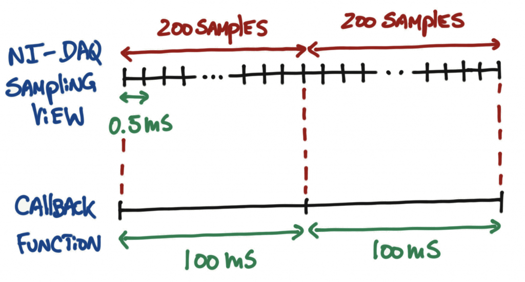
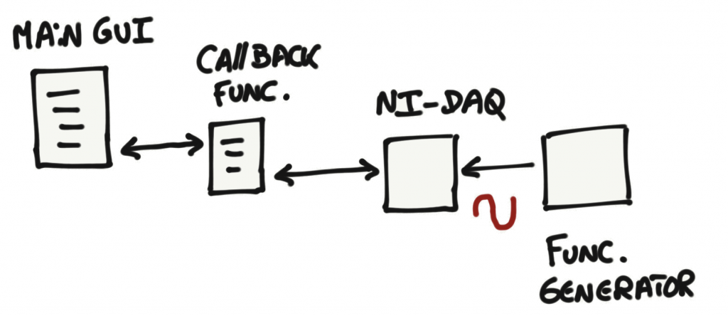
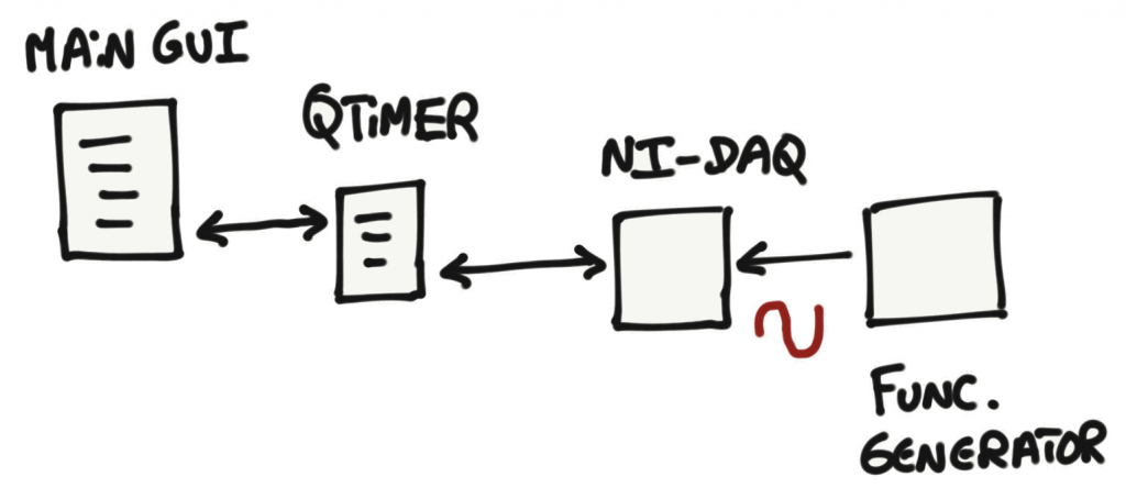
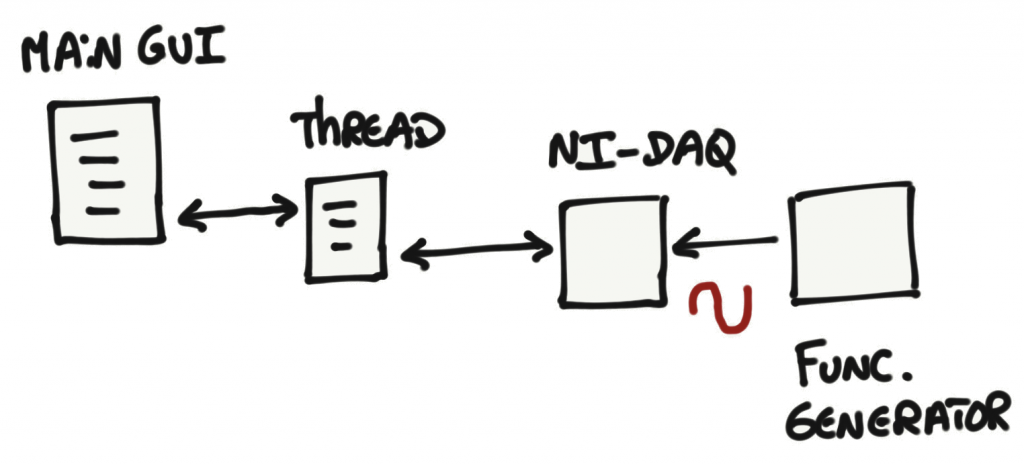
The code below runs in a normal Operating System, using the NI-DAQ ability to acquire samples at faster rates and deliver those samples to your application that runs at manageable timings at the user level. We can abstract this concept with the diagram below.
- We will set up the NI-DAQ to acquire at a sampling rate of 2kHz (0.5ms) and after collecting 200 samples we can then use the user level program to get the data and render or process it at a rate of 10Hz (100ms).
The code below is also done in python to make it easier to understand, follow and reproduce. However, similar concepts apply if you do the code in another programming languages (e.g.: C/C++, C#, or Java).
I will be showing 3 different approaches to acquire the data from the NI-DAQ:
- NI callback functions (Link)
- QTimers from Qt (Link)
- Threads: make sure that you read [REF 5] if you are not familiar with threads in Python
The beginning of the code for all 3 approaches is exactly the same:
- Create an NI Task
- Configure the NI Task
- Configure sampling rate and acquisition type
- Create a stream reader object
After this point is when each approach sets up the task that gets the information from the NI-DAQ accordingly.
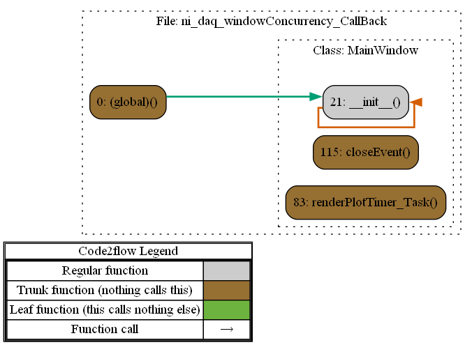
NI Callback Function
I hope the comments throughout the code help understanding what is going on.
- Everything from line 25 to 70 is the same for each approach.
- On line 74, we create the NI callback function that is going to be triggered based on the number of samples that you want. In our case it will be 200 samples. The callback function to call is called renderPlotTimer_Task.
- The code inside renderPlotTimer_Task is just an example of what is possible to do with the acquired data.
- On line 109, the code will plot the AC component of the signal
- On line 108, the code will plot the DC component of the signal. This is an example of a simple DSP algorithm (average value of a signal).
- Have in mind, the way the code is written, you can't have line 108 and 109 at the same time. Comment and uncomment the code according to what you want to see.
import sys
import random
from collections import deque

import numpy as np
from PyQt6 import QtCore, QtGui, QtWidgets, uic
from PyQt6.QtWidgets import QApplication, QLabel, QInputDialog, QMessageBox

import nidaqmx
from nidaqmx import constants, system
from nidaqmx.constants import Edge, AcquisitionType
from nidaqmx import stream_readers

from nidaqmx.stream_readers import AnalogSingleChannelReader

from pyqtgraph import PlotWidget
import pyqtgraph as pg


class MainWindow(QtWidgets.QMainWindow):
    def __init__(self, *args, **kwargs):
        super().__init__(*args, **kwargs)
        uic.loadUi("ni_daq_windowConcurrency.ui", self)

        # Initialize Plot
        # -----------------
        self.widgetPlot.setTitle("Analog Data Test")
        self.widgetPlot.setLabel('left', 'Voltage (V)')
        self.widgetPlot.setLabel('bottom', 'Time (s)')
        self.widgetPlot.setBackground('w')
        self.widgetPlot.setYRange(-6.0, 6.0, padding=0)

        self.dat = deque()
        self.xTime = deque()
        self.xCounter = 0
        self.maxLen = 200
        self.xValues = np.arange(1, 201)  # change the size based on self.samples_per_channel
        self.xCounterArray = 0

        self.curve1 = self.widgetPlot.plot(pen='r')

        # Initialize DAQ
        # ----------------
        self.deviceName = "6002_Dev2/ai0"

        # Create NIDAQmx Task
        self.aiDAQTask = nidaqmx.Task()

        # Configure NIDAQms Task
        self.aiDAQTask.ai_channels.add_ai_voltage_chan(self.deviceName, "",
                                                       nidaqmx.constants.TerminalConfiguration.RSE,
                                                       -5.0, 5.0,
                                                       nidaqmx.constants.VoltageUnits.VOLTS, None)

        # Configure sampling rate and acquisition type (Continuous)
        self.fs = 2000
        self.samplingRate = 0.1  # msecs

        self.samples_per_channel = int(self.fs * self.samplingRate)  # 2000 * 0.1 = 200 samples
        self.num_channels = 1

        self.aiDAQTask.timing.cfg_samp_clk_timing(self.fs, None, nidaqmx.constants.Edge.RISING,
                                                  nidaqmx.constants.AcquisitionType.CONTINUOUS,
                                                  self.samples_per_channel * self.num_channels)

        # Create stream reader object
        self.in_stream_reader = AnalogSingleChannelReader(self.aiDAQTask.in_stream)

        # Initialize data 1D array of input analog samples
        self.in_stream_array = np.zeros(self.samples_per_channel, dtype=np.float64)

        # Initialize NI Callback Function
        # ------------------
        self.aiDAQTask.register_every_n_samples_acquired_into_buffer_event(self.samples_per_channel,
                                                                           self.renderPlotTimer_Task)

        # Start Timer and DAQ
        # --------------------
        self.aiDAQTask.start()

    # -----------------------------------

    def renderPlotTimer_Task(self, task_handle, every_n_samples_event_type, number_of_samples, callback_data):
        if len(self.dat) > self.maxLen:
            self.dat.popleft()  # remove oldest
            self.xTime.popleft()

        # Update time axis
        self.xCounter += self.samplingRate
        self.xTime.append(self.xCounter)

        # Update time axis for array of data
        self.xValues += 200*self.xCounterArray
        self.xCounterArray += 1

        # Read Analog values from NI DAQ
        self.in_stream_reader.read_many_sample(self.in_stream_array,
                                               number_of_samples_per_channel=self.samples_per_channel,
                                               timeout=10.0)

        np_values = np.array(self.in_stream_array)
        #print(len(np_values))
        mean_value = np.mean(np_values)

        # Append value to data
        self.dat.append(mean_value)

        #self.curve1.setData(self.xTime, self.dat)  # plots DC component
        self.curve1.setData(self.xValues, np_values)  # plots AC component

        return 0

    # -------------------------------------------------

    def closeEvent(self, *args, **kwargs):
        self.aiDAQTask.stop()
        self.aiDAQTask.close()


if __name__ == "__main__":
    app = QApplication(sys.argv)
    win = MainWindow()
    win.show()
    sys.exit(app.exec())
QTimers
If you were able to follow the NI callback function code, you will notice that the code below is not that much different.
- Now instead of creating an NI callback function, we create an QTimer (Line 75 to 77).
- The interval of the QTimer is set to 100ms.
- renderPlotTimer_Task is exactly the same code as in the previous section
Note: according to the manual the QTimer setInterval function accepts an integer value that represents the interval in milliseconds. For some reason, in order for my QTimer to run at proper timings I need to use a float number. I am using Python 3.7 and PyQt6. Just heads up if you are using a more recent version of Python and things got solved and you need to use an integer number.

import sys
import random
from collections import deque

import numpy as np
from PyQt6 import QtCore, QtGui, QtWidgets, uic
from PyQt6.QtWidgets import QApplication

import nidaqmx
from nidaqmx import constants, system
from nidaqmx.constants import AcquisitionType
from nidaqmx import stream_readers

from nidaqmx.stream_readers import AnalogSingleChannelReader

from pyqtgraph import PlotWidget
import pyqtgraph as pg


class MainWindow(QtWidgets.QMainWindow):
    def __init__(self, *args, **kwargs):
        super().__init__(*args, **kwargs)
        uic.loadUi("ni_daq_windowConcurrency.ui", self)

        # Initialize Plot
        # -----------------
        self.widgetPlot.setTitle("Analog Data Test")
        self.widgetPlot.setLabel('left', 'Voltage (V)')
        self.widgetPlot.setLabel('bottom', 'Time (s)')
        self.widgetPlot.setBackground('w')
        self.widgetPlot.setYRange(-6.0, 6.0, padding=0)

        self.dat = deque()
        self.xTime = deque()
        self.xCounter = 0
        self.maxLen = 200
        self.xValues = np.arange(1, 201)  # change the size based on self.samples_per_channel
        self.xCounterArray = 0

        self.curve1 = self.widgetPlot.plot(pen='r')

        # Initialize DAQ
        # ----------------
        self.deviceName = "6002_Dev2/ai0"

        # Create NIDAQmx Task
        self.aiDAQTask = nidaqmx.Task()

        # Configure NIDAQms Task
        self.aiDAQTask.ai_channels.add_ai_voltage_chan(self.deviceName, "",
                                                       nidaqmx.constants.TerminalConfiguration.RSE,
                                                       -5.0, 5.0,
                                                       nidaqmx.constants.VoltageUnits.VOLTS, None)

        # Configure sampling rate and acquisition type (Continuous)
        self.fs = 2000
        self.samplingRate = 0.1  # msecs

        self.samplingRate_s = self.samplingRate #/ 1000
        self.samples_per_channel = int(self.fs * self.samplingRate_s)
        self.num_channels = 1

        self.aiDAQTask.timing.cfg_samp_clk_timing(self.fs, None, nidaqmx.constants.Edge.RISING,
                                                  nidaqmx.constants.AcquisitionType.CONTINUOUS,
                                                  self.samples_per_channel * self.num_channels)

        # Create stream reader object
        self.in_stream_reader = AnalogSingleChannelReader(self.aiDAQTask.in_stream)

        # Initialize data 1D array of input analog samples
        self.in_stream_array = np.zeros(self.samples_per_channel, dtype=np.float64)

        # Initialize Qtimer
        # ------------------
        self.renderPlotTimer = QtCore.QTimer()
        self.renderPlotTimer.setInterval(self.samplingRate)
        self.renderPlotTimer.timeout.connect(self.renderPlotTimer_Task)

        # Start Timer and DAQ
        # --------------------
        self.aiDAQTask.start()
        self.renderPlotTimer.start()

    # -----------------------------------

    def renderPlotTimer_Task(self):
        if len(self.dat) > self.maxLen:
            self.dat.popleft()  # remove oldest
            self.xTime.popleft()

        # Update time axis
        self.xCounter += self.samplingRate #/ 1000
        self.xTime.append(self.xCounter)

        # Update time axis for array of data
        self.xValues += 200 * self.xCounterArray
        self.xCounterArray += 1

        # Read Analog values from NI DAQ
        self.in_stream_reader.read_many_sample(self.in_stream_array,
                                               number_of_samples_per_channel=self.samples_per_channel,
                                               timeout=10.0)

        np_values = np.array(self.in_stream_array)
        #print(len(np_values))
        mean_value = np.mean(np_values)

        # Append value to data
        self.dat.append(mean_value)

        # Plot data
        #self.curve1.setData(self.xTime, self.dat)
        self.curve1.setData(self.xValues, np_values)  # plots AC component

    # -------------------------------------------------

    def closeEvent(self, *args, **kwargs):
        self.aiDAQTask.stop()
        self.aiDAQTask.close()
        self.renderPlotTimer.stop()


if __name__ == "__main__":
    app = QApplication(sys.argv)
    win = MainWindow()
    win.show()
    sys.exit(app.exec())
Threads
I left the threads as the last example just because the code to set up a thread can be a bit overwhelming if you are not familiar with it. There are also a couple of different ways to create threads and implement the communication between threads and the main GUI.
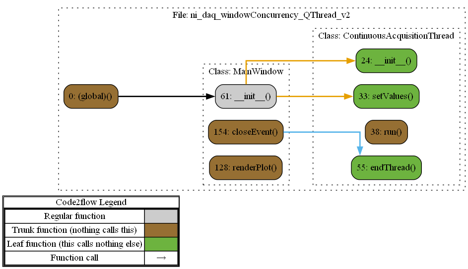
The code below implements Qt signals & slots to transfer information between the thread and the main GUI.
- Since the plotting is done on the main GUI, I now establish a signal and slot communication between the thread and the main GUI (Line 120).
- The thread generates a signal (at Line 49) when data is available from the DAQ, and the function connected to that signal renderPlot (on Line 128) is executed as a normal function call, totally independent of any GUI event loop.
import sys
import random
from collections import deque

import numpy as np
from PyQt6 import QtCore, QtGui, QtWidgets, uic
from PyQt6.QtWidgets import QApplication, QLabel, QInputDialog, QMessageBox
from PyQt6.QtCore import QThread, QObject, pyqtSignal, pyqtSlot

import nidaqmx
from nidaqmx import constants, system
from nidaqmx.constants import Edge, AcquisitionType
from nidaqmx import stream_readers

from nidaqmx.stream_readers import AnalogSingleChannelReader

from pyqtgraph import PlotWidget
import pyqtgraph as pg


class ContinuousAcquisitionThread(QThread):
    signal = pyqtSignal(object)

    def __init__(self):
        super(ContinuousAcquisitionThread, self).__init__()
        # Initialize aux variables
        self.endFlag = False

        self.in_stream_reader = None
        self.in_stream_array = None
        self.samples_per_channel = None

    def setValues(self, in_stream_reader, in_stream_array, samples_per_channel):
        self.in_stream_reader = in_stream_reader
        self.in_stream_array = in_stream_array
        self.samples_per_channel = samples_per_channel

    def run(self):

        while True:

            # Read Analog values from NI DAQ
            self.in_stream_reader.read_many_sample(self.in_stream_array,
                                                   number_of_samples_per_channel=self.samples_per_channel,
                                                   timeout=10.0)

            np_values = np.array(self.in_stream_array)

            self.signal.emit(np_values)

            if self.endFlag:
                print("Thread done.")
                break

    def endThread(self):
        self.endFlag = True


class MainWindow(QtWidgets.QMainWindow):

    def __init__(self, *args, **kwargs):
        super().__init__(*args, **kwargs)
        uic.loadUi("ni_daq_windowConcurrency.ui", self)

        # Initialize Plot
        # -----------------
        self.widgetPlot.setTitle("Analog Data Test")
        self.widgetPlot.setLabel('left', 'Voltage (V)')
        self.widgetPlot.setLabel('bottom', 'Time (s)')
        self.widgetPlot.setBackground('w')
        self.widgetPlot.setYRange(-6.0, 6.0, padding=0)

        self.dat = deque()
        self.xTime = deque()
        self.xCounter = 0
        self.maxLen = 100
        self.xValues = np.arange(1, 201)  # change the size based on self.samples_per_channel
        self.xCounterArray = 0

        self.curve1 = self.widgetPlot.plot(pen='r')

        # Initialize DAQ
        # ----------------
        self.deviceName = "6002_Dev2/ai0"

        # Create NIDAQmx Task
        self.aiDAQTask = nidaqmx.Task()

        # Configure NIDAQms Task
        self.aiDAQTask.ai_channels.add_ai_voltage_chan(self.deviceName, "",
                                                       nidaqmx.constants.TerminalConfiguration.RSE,
                                                       -5.0, 5.0,
                                                       nidaqmx.constants.VoltageUnits.VOLTS, None)

        # Configure sampling rate and acquisition type (Continuous)
        self.fs = 2000
        self.samplingRate = 0.1  # msecs

        self.samples_per_channel = int(self.fs * self.samplingRate)
        self.num_channels = 1

        self.aiDAQTask.timing.cfg_samp_clk_timing(self.fs, None, nidaqmx.constants.Edge.RISING,
                                                  nidaqmx.constants.AcquisitionType.CONTINUOUS,
                                                  self.samples_per_channel * self.num_channels)

        # Create stream reader object
        self.in_stream_reader = AnalogSingleChannelReader(self.aiDAQTask.in_stream)

        # Initialize data 1D array of input analog samples
        self.in_stream_array = np.zeros(self.samples_per_channel, dtype=np.float64)

        # Initialize QThread
        # ------------------
        self.worker_ContinuousAcquisitionThread = ContinuousAcquisitionThread()

        self.worker_ContinuousAcquisitionThread.setValues(in_stream_reader=self.in_stream_reader,
                                                          in_stream_array=self.in_stream_array,
                                                          samples_per_channel=self.samples_per_channel)

        self.worker_ContinuousAcquisitionThread.signal.connect(self.renderPlot)

        # Start QThread
        # --------------------
        self.worker_ContinuousAcquisitionThread.start()

    # -------------------------------------------------

    def renderPlot(self, msg):
        if len(self.dat) > self.maxLen:
            self.dat.popleft()  # remove oldest
            self.xTime.popleft()

        # Update time axis
        self.xCounter += self.samplingRate
        self.xTime.append(self.xCounter)

        # Update time axis for array of data
        self.xValues += 200 * self.xCounterArray
        self.xCounterArray += 1

        # Read Analog values from QTSignal
        np_values = msg
        mean_value = np.mean(np_values)

        # Append value to data
        self.dat.append(mean_value)

        # Plot data
        #self.curve1.setData(self.xTime, self.dat)
        self.curve1.setData(self.xValues, np_values)  # plots AC component

    # -------------------------------------------------

    def closeEvent(self, *args, **kwargs):
        self.worker_ContinuousAcquisitionThread.endThread()

        self.aiDAQTask.stop()
        self.aiDAQTask.close()


if __name__ == "__main__":
    app = QApplication(sys.argv)
    win = MainWindow()
    win.show()
    sys.exit(app.exec())
In summary:
- Which technique should you use? Use the technique that works best with the rest of the code that you are developing.
- In terms of being deterministic, the 3 solutions rely on the NI-DAQ to do the heavy lifting, and they are all running at manageable timings at the user level.
- Callbacks and Threads can be used in a GUI or console application
- QTimers are only available with PyQt but they can also be used in a console application as long as you create a QtWidgets object and initiate the timer accordingly. I will leave the skeleton code for this case under the Python Files section -> ni_daq_consoleConcurrency_QTimer.py.
Besides QTimers and QThreads, Qt offers other techniques to work with threads (e.g.: QThreadPool, QRunnable, QtConcurrent, and WorkerScript). Check this link if you are interested to understand how to choose an appropriate approach for your application.
NI-DAQ Functions Used
- nidaqmx.Task
- ai_channels.add_ai_voltage_chan
- timing.cfg_samp_clk_timing
- AnalogSingleChannelReader
- register_every_n_samples_acquired_into_buffer_event
- read_many_sample
- start
- stop
- close
Python Files
References
- [REF 1] "PySDR: A Guide to SDR and DSP using Python", PySDR [Article]
- [REF 2] "Time and Frequency Domains", Mike X Cohen YouTube Channel [Video]
- [REF 3] "Aliasing", Wikipedia [Article]
- [REF 4] "Sample Rate: How to Pick the Right One", Endaq [Article]
- [REF 5] "An Intro to Threading in Python", Real Python [Article]
- [REF 6] "Anti-aliasing Filter Design and Applications in Sampling", Cadence [Article]
- [REF 7] "Threading Basics", Qt Documentation [Article]
- [REF 8] "Multithreading Technologies in Qt", Qt Documentation [Article]