LTSpice FFT
FFT
The reference videos at the end of this article do a fantastic job explaining in detail how to use the FFT in LTSpice, and how to setup the environment variables in order to reduce the effects of compression on the frequency spectrum. I recommend checking those references out to get additional information that is not covered in this article.
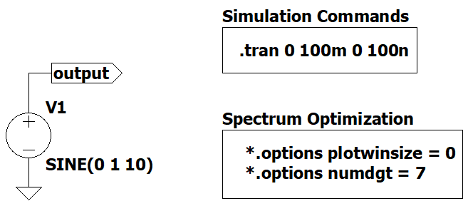
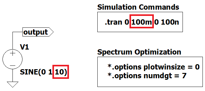
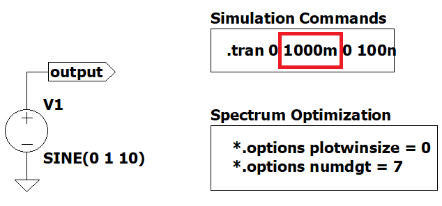
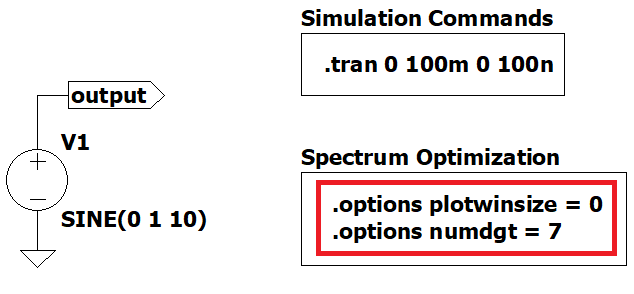
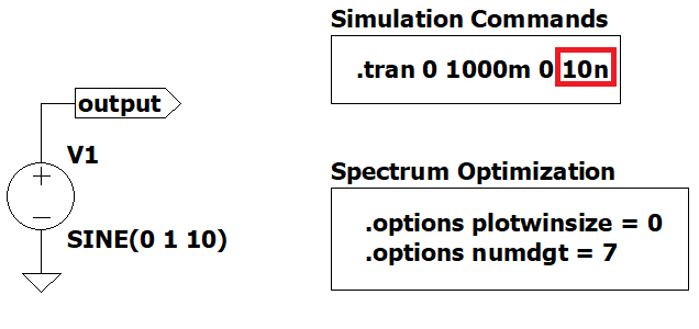
We will be using Figure 1 as an example to change some .options and .tran parameters and see what happens in the spectrum.
Understanding .tran Plot
The first step to understand the FFT in LTspice is to understand the relationship between the .tran command and the minimum frequency of the signal of interest.

When we set .tran 0 100m 0 100n, the minimum waveform that we can display in time is (1/<Tstop>) = (1/0.1) 10 Hz (one full cycle).
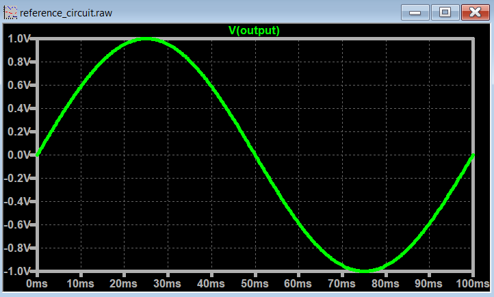
If the minimum frequency of your signal is smaller than 10Hz, the time plot will not display a full cycle of that waveform.
This can be problematic. You need at least set the .tran <Tstop> parameter to the minimum frequency of your signal, otherwise you will get weird results during an FFT plot analysis.
Understanding the FFT Plot
We will see very soon on how to plot FFTs with LTSpice.
The important part to retain in this section is to have in mind that the x-axis will always show 5 decades of frequencies.
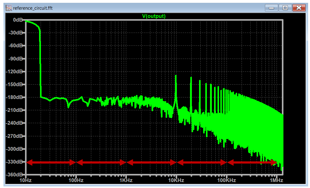
And we can change this range of frequencies based on the .tran <Tstop> parameter. More on this shortly.
Spectrum Optimization Parameters Off
Let's plot the FFT with the spectrum optimization parameters off and keep the .tran <Tstop> parameter equal to the frequency of the signal (10Hz -> 100ms).
After plotting the time response, right click on the plot, go to "view->FFT". For now leave all the parameters from the FFT dialog menu by default and press ok.
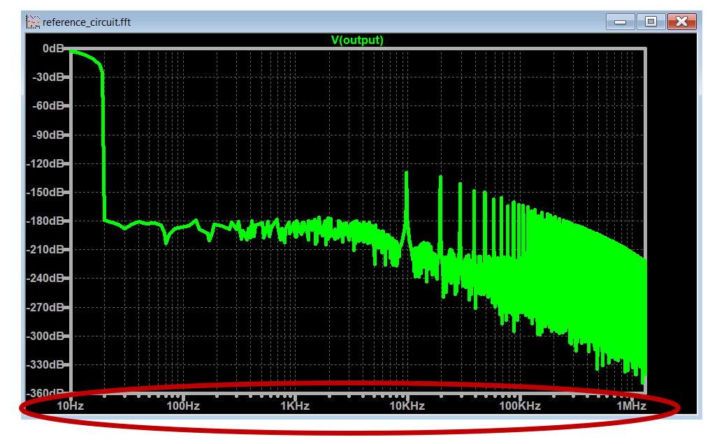
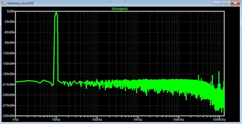
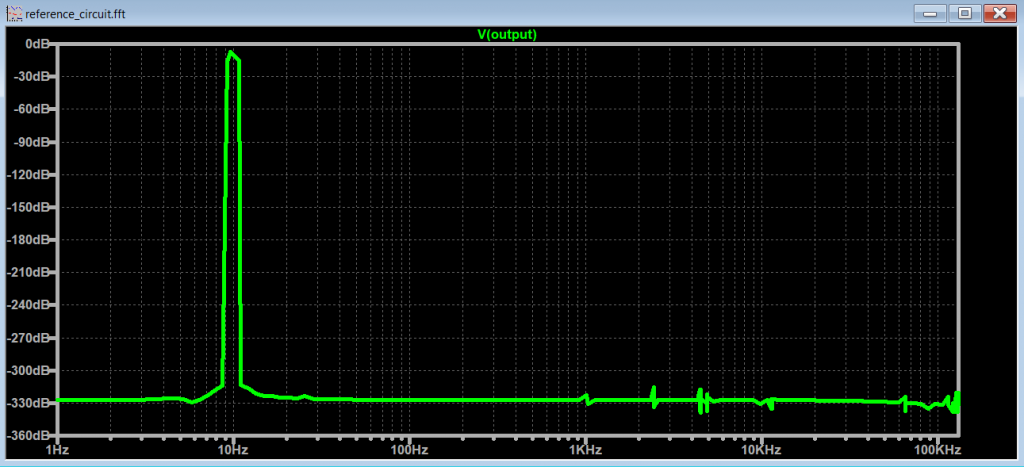
It is interesting to notice that the minimum frequency that you see on the spectrum is 10Hz which corresponds to the .tran <Tstop> (100ms) equivalent frequency. The expected sinusoidal spike at 10Hz is there but not completely visible.
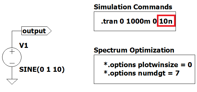
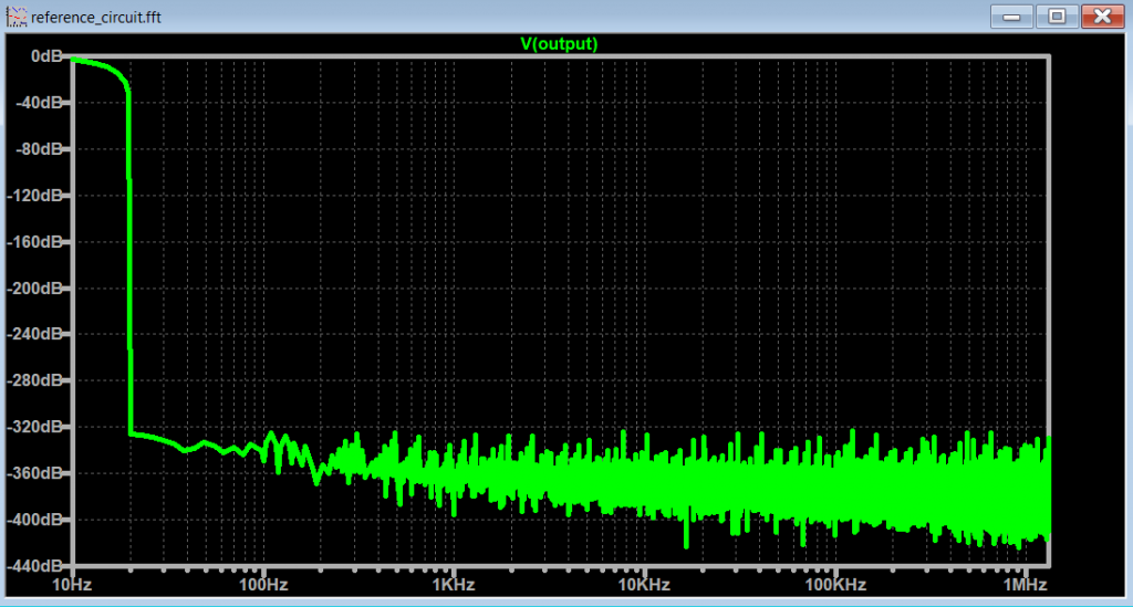
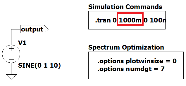
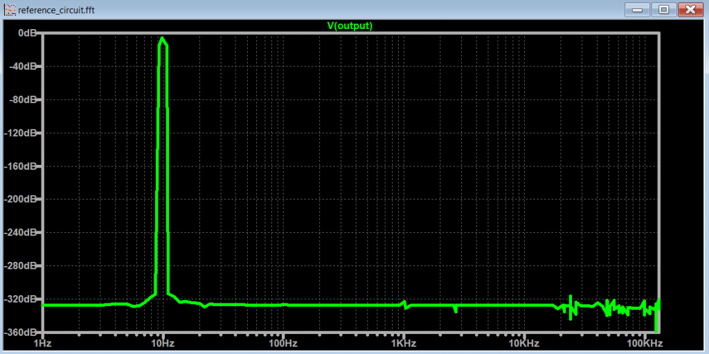
If we keep the frequency of the signal the same and increase the .tran <Tstop> to 1000ms, we get the following FFT:
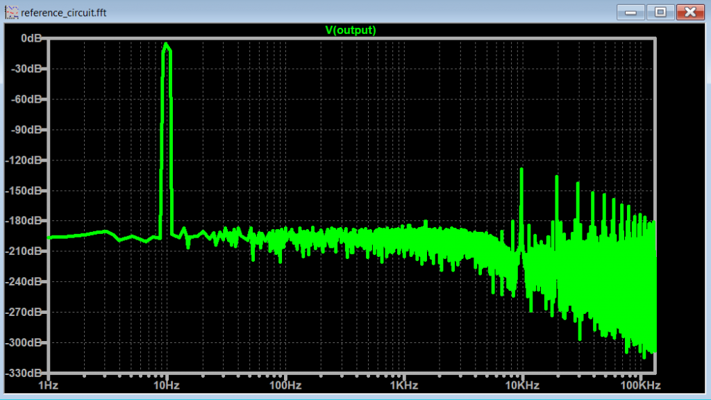
Notice now that the minimum frequency on the spectrum is (1/<Tstop>) = (1/1000ms) = 1 Hz. And no surprise here, we can see the peak of the sinusoidal wave at 10Hz way better.
Note: the spectrum for the higher frequency content is still "suffering" from compression that the FFT in LTSpice implements. We will find solutions to fix this soon.
Spectrum Optimization Parameters Off + Decrease .tran timestep
An immediate way to improve the higher frequency content of the FFT, is to decrease the .tran <Tmaxstep>. This means that the FFT algorithm will use more points to compute the FFT. The downside is that we increase the simulation time considerably.
If we want plot FFTs without taking too much time simulating, we will need to use another solution.
Spectrum Optimization Parameters On
Let's go back to the original circuit in Figure 1, and uncomment the spectrum optimization spice commands and run the FFT with these settings enabled.
Notice that just by including those .options during simulation, Plot 8 spectrum improves compared to Plot 5.
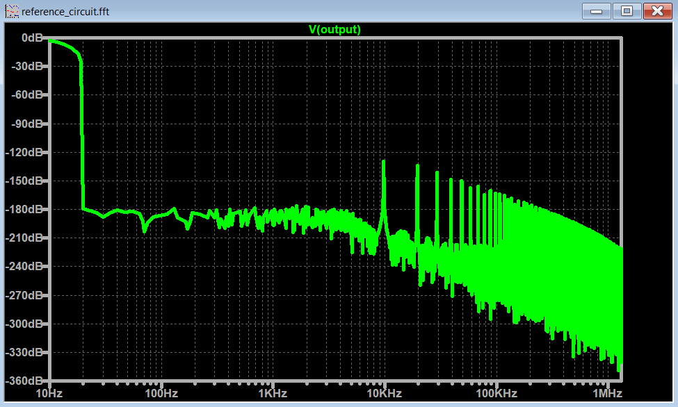
And if we change the .tran <Tstop> to 1000ms, we get even better results.
And finally combining the .options parameters and decrease the .tran <Tmaxstep>, we get the following FFT:
At this point, for this particular example, there is no benefit by increasing the number of points on the resultant FFT.
Incorrect .tran setup & FFT
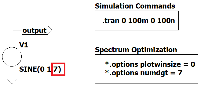
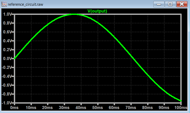
Let's go back to Figure 3 and observe the spectrum when the frequency of our signal is lower than the minimum frequency used for .tran <Tstop>:

Notice on how it is hard to make sense of the spectrum, mainly because the frequency of interest (7 Hz) is smaller than the minimum frequency on the x-axis (10 Hz). It is important to adjust the .tran <Tstop> parameter to fully represent the signals that we are trying to visualize with the FFT.
Other Examples
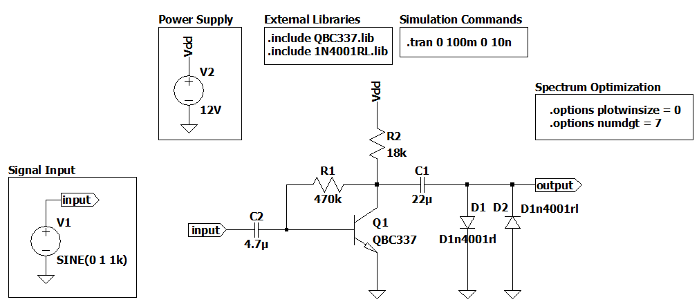
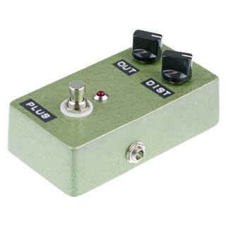
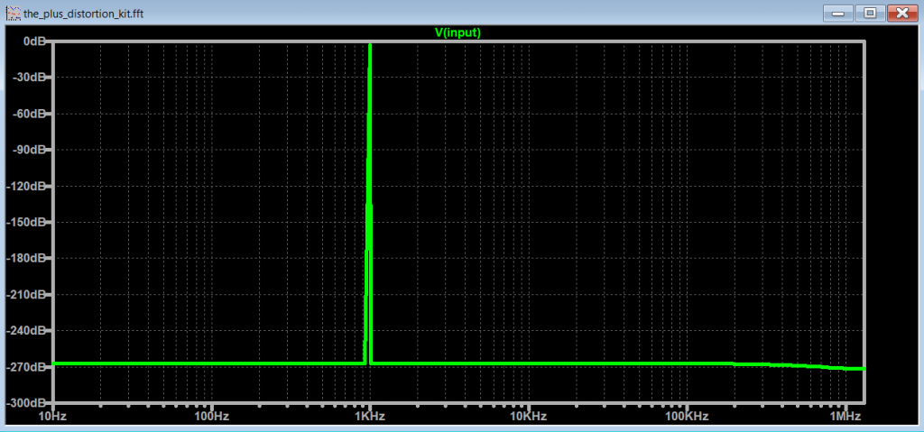
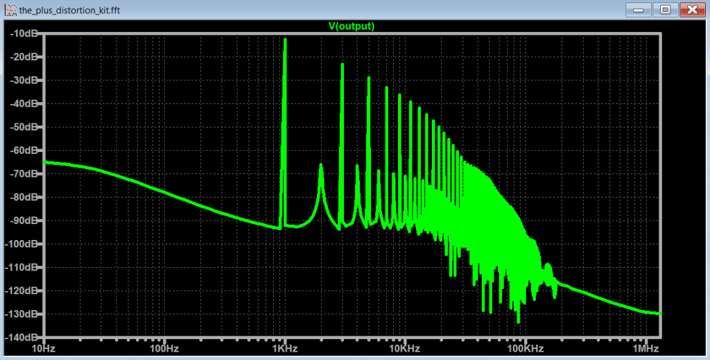
Simple Distortion Guitar Pedal
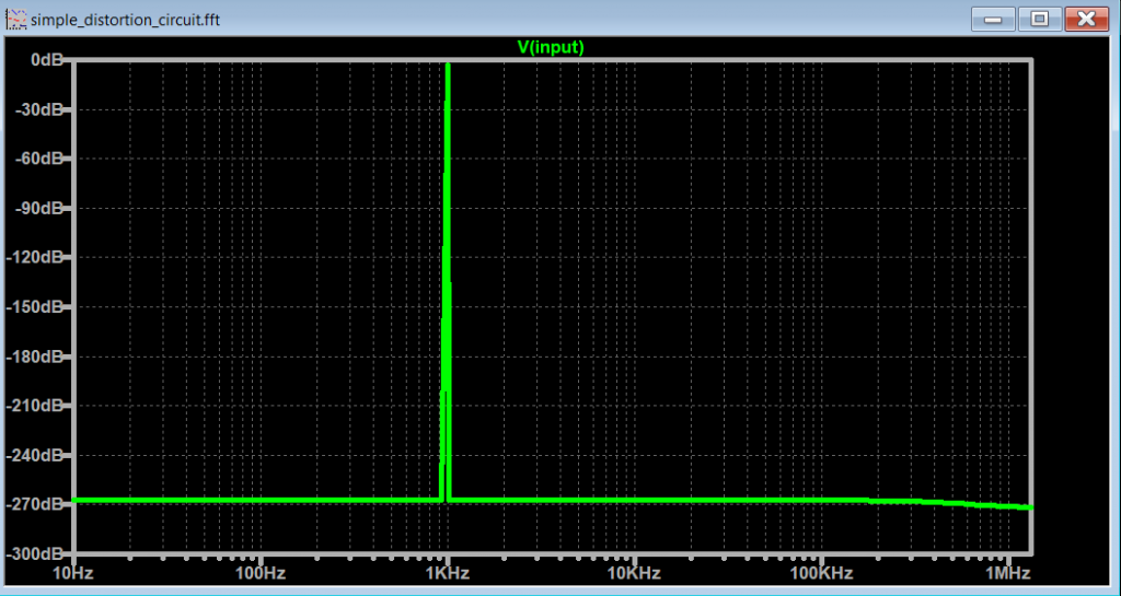
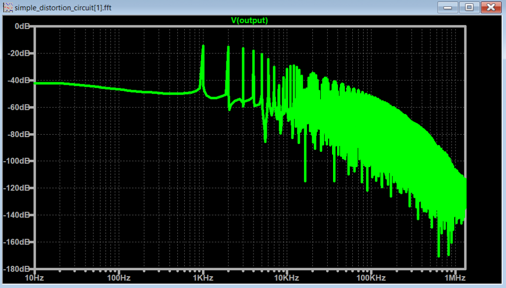
The Plus - Distortion kit
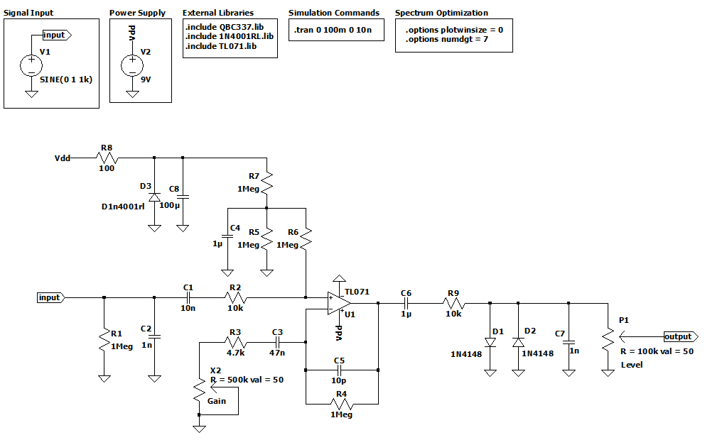
LTSpice Simulation Files
Spice Components
Directions: Download the spice model and place it in the same project folder that you are working.
References
- [Ref 1] “LTspice #13: Performing and Cleaning Up An FFT“, trevortjes YouTube Channel [Video]
- [Ref 2] “LTspice Tutorial - Ep6 Basics of FFT analysis and .four statement“, FesZ Electronics YouTube Channel [Video]
- [Ref 3] “Frequency Analysis Using FFT“, cytechglobal - Analog Devices [Article]