LTSpice Variable Parameters
Introduction
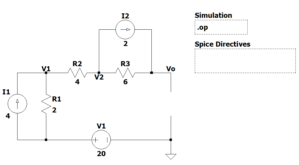
During homework exercises or labs, sometimes you need to analyze the circuits for different components values. Let's use the circuit below as our first example:
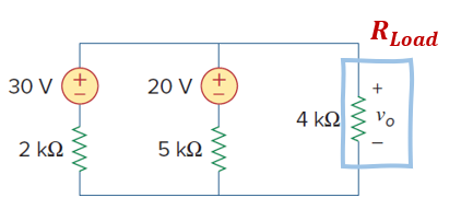
Let's say we want to analyze the output voltage (Vo) for several different values of a load resistor (RL).
Let's build the LTSpice circuit with the original RL value first.
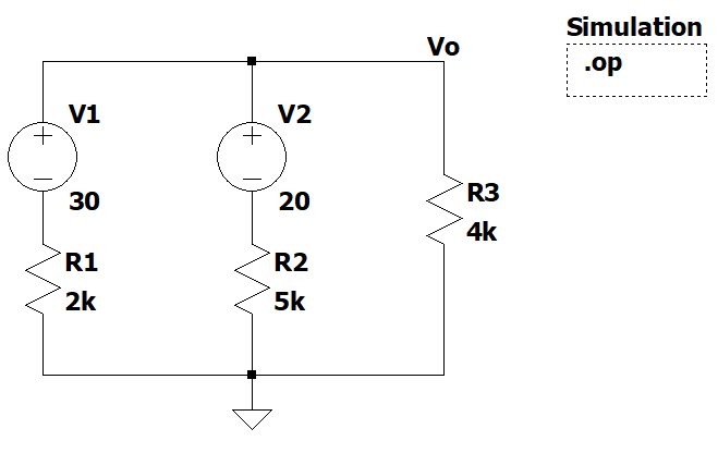
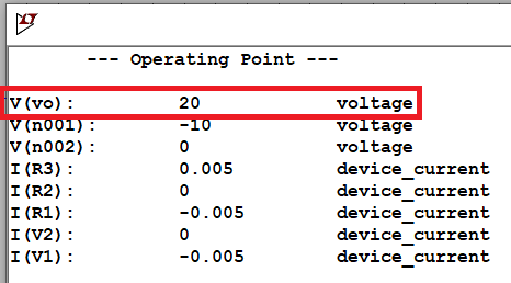
Since we don't have AC signals in this circuit, it is all DC analysis, we are going to simulate the DC operating point of the circuit using the ".op" simulation command.
Now let's say that we want to analyze Vo for 10 different types of RL. You can change them manually, which will take some time, but you can also set a variable parameter for RL and change it's value automatically.
.param Command -> User-Defined Variable
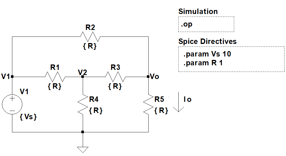
Let's start by creating a user-defined variable in LTSpice. This is useful for associating a name with a value for the sake of clarity and parameterizing your circuits.
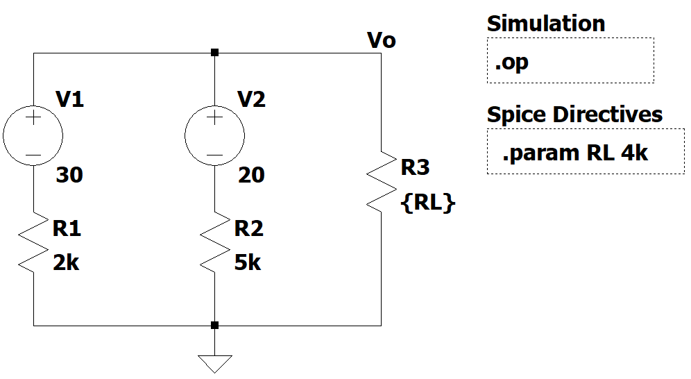
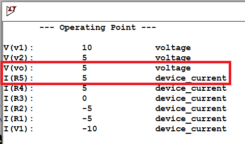
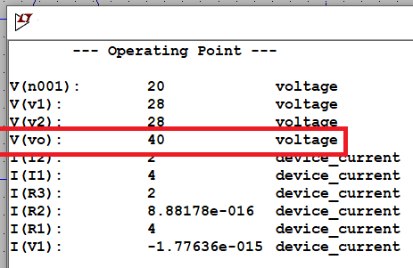
Enclose your variable names in curly braces, in this case {RL}, and then set the SPICE directive ".param" with the desired valued for your variable name. Run the simulation and you should get the same results as in Figure 3.
.step Command -> List of Parameters
Now let's change the values of RL automatically and analyze the results. One way to achieve this is to create a list of desired values to test.
Note: "*" is used as a comment in SPICE. Any SPICE directive with a "*" in front of it, will not run during simulation.
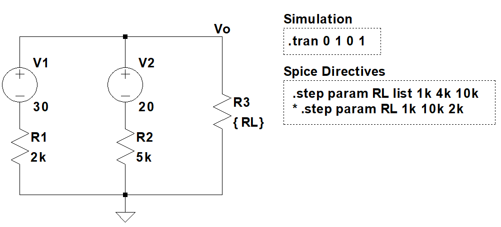
We are commenting the second Spice directive for now.
The command ".step" performs parameters sweeps. The ".step" command has different flavors. One of those flavors is the ability to include a list of values for your variable name.
The DC operating point, ".op" simulation doesn't output an answer with respect to time. To see the results with respect to time, we need to change the simulation type to ".tran", transient analysis.
On the output graph, add the signals of interest to that graph (in this case Vo) and add a cursor. If you move the keys up and down in your keyboard you will be able to change between all the different answers.
To know which value of RL corresponds to that particular answer, right click with your mouse on top of it and a pop up window will show you the respective parameter value.
.step Command -> Increasing Order
Another way to simulate a set of values at the same time is to use the increasing order option of the ".step" command. We comment the first SPICE directive line and uncomment the second line.
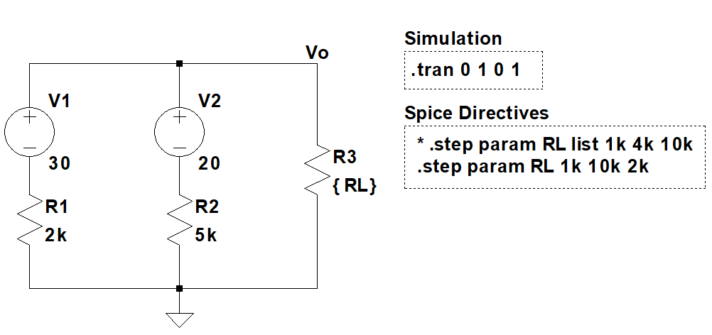
For this particular example, the increasing order option goes from 1k to 10k in increment steps of 2k. After running the simulation, you can iterate through all the answers the same way as we did in Figure 6 and 7.
Applications
So far, we saw how to apply variable parameters to find current and voltages for components that can have multiple values, and use the ".tran" simulation command to check the answers in terms of time.
Another use of variable parameters can be to find the maximum power transferred to a load.
Maximum Power Transfer
In many practical situations, a circuit is designed to provide power to a load, and sometimes it is desirable to maximize the power delivered to that same load (normally called RL).
To find the maximum power transferred to RL, we can declare RL as a variable resistor but this time we will run the DC Operating ".op" simulation to get an answer for a list of RL values.
Let's find the value of RL that corresponds to the the maximum power transfer to RL in the circuit from Figure 4.
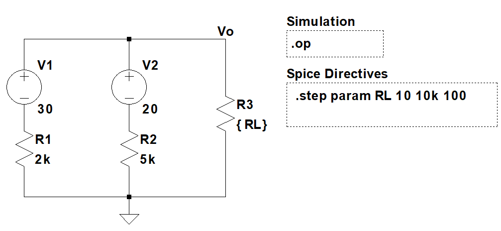
The only change that we need to make is to add a set of values for the variable parameter RL. It would take time to add and adjust values using the ".step" list method. However, with the ".step" increase order method that can be done faster. Here we are simulating RL from 10Ω to 10kΩ in steps of 100Ω
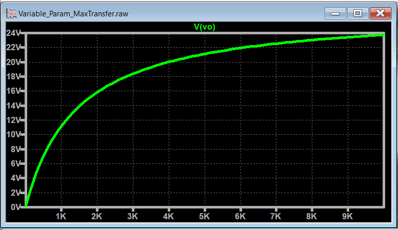
After running the simulation we get the following plot with Vo vs RL.
We are almost there. Now let's add a second trace on the graph and add the following SPICE expression, "V(vo)*I(R3)", to calculate the power across R3 = RL.
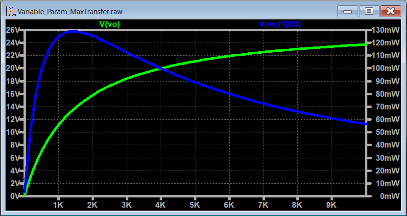
Add a cursor to the graph and check the value of RL that gives you the maximum power value (the global maximum of the power curve).
Other Examples
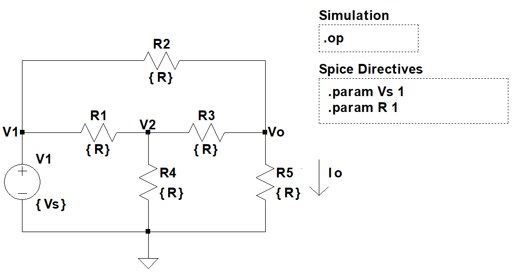
Example 1
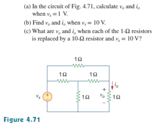
LTSpice Solutions
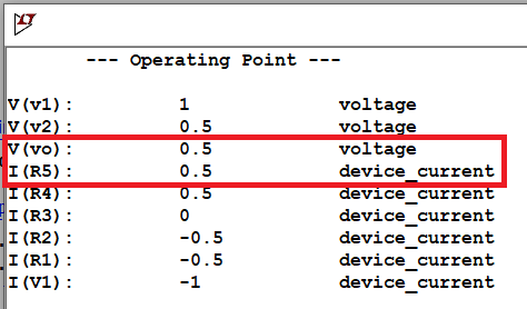
One Parameter
(a)
(b)
(c)

Multiple Parameters
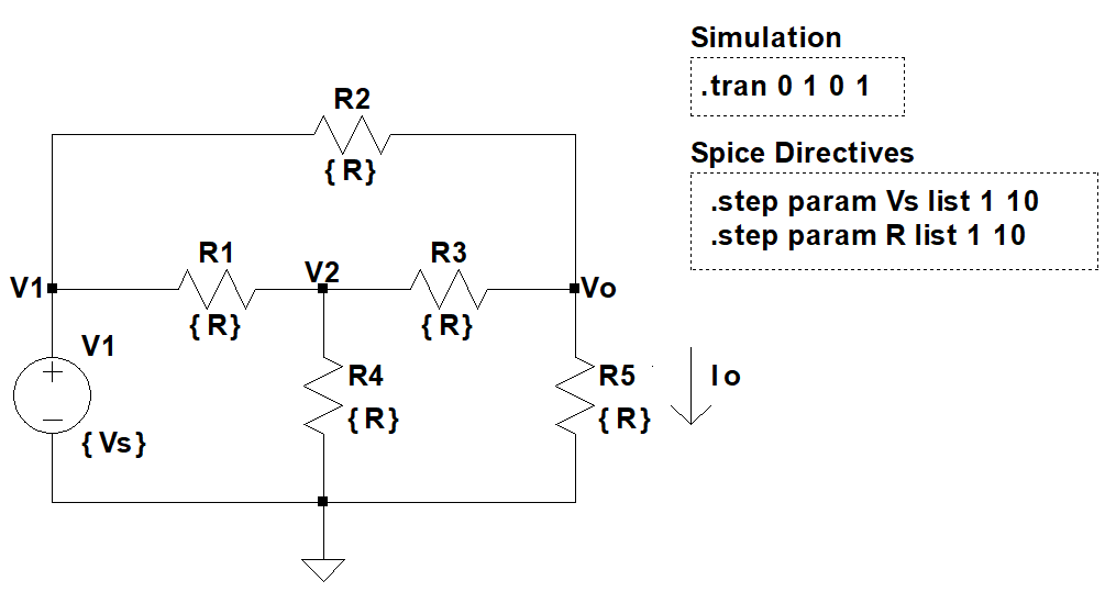
If you simulate multiple parameters at the same time, LTSpice will compute all possible combinations between those parameters.
For this exercise, we have 2 variable parameters, Vs and R, which gives a total of 4 possible solutions.
Note: For this approach to run without errors, make sure that the size of the list is equal to number of variable parameters.
To plot a specific answer, right click on the graph, go to View and select "Select Steps". From the list of options select the desired one.
Example 2
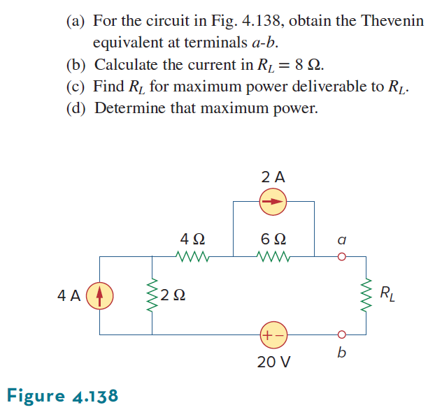
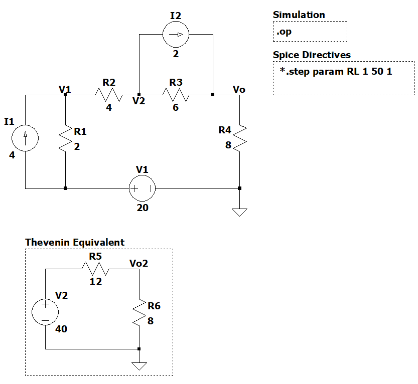
We are going to work on this exercise in a slightly different order than the one asked by the exercise. We are going to find c) and d) first and then find the equivalent Thevenin a), and at last we will find the current in RL for b).
Let's build the circuit in LTSpice. It is important to understand that if you place the ground reference in a different point you are going to get different results.
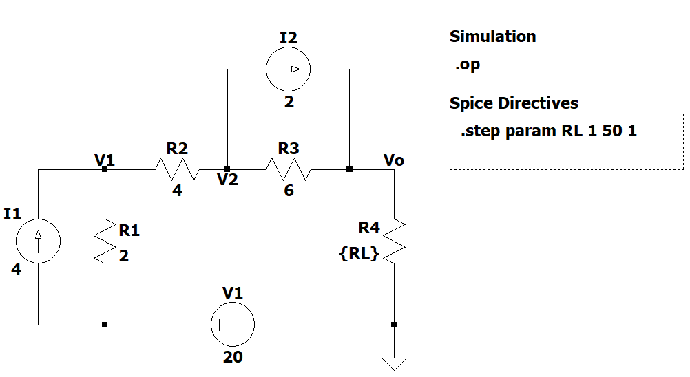
Let's get RL for the maximum power.
(c) and (d) answer -> RL = 12Ω for P = 33.33 W
To answer (a), we need the open circuit voltage (Voc) and the Thevenin resistance (Rth). The Thevenin resistance is equal to RL for maximum power, in this case Rth = 12Ω.
The open circuit voltage is Voc = 40 V.
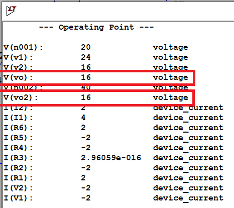
Finally to find the answer to b), let's have both circuits side to side with RL = 8Ω
LTSpice Simulation Files
- Variable Parameter Example
- Example 1 .op Simulation (One Parameter)
- Example 1 .tran Simulation (Multiple Parameters)
- Variable Parameter Maximum Power Example
- Example 2 (Maximum Power Transfer)
References
- [Ref 1] "LTspice: Using the .STEP Command to Perform Repeated Analysis", Analog Devices [Article]
- [Ref 2] "LTspice: Stepping Parameters", Analog Devices [Video]
- [Ref 3] "LTSpice Maximum Power Transfer Tutorial", DMExplains YouTube Channel [Video]