Single Analog Input – Demand
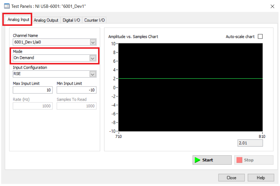
For this article I am going to show how to implement the on demand single analog input mode from the test panel NI-MAX software. I encourage to test this mode first using the NI-MAX software in order to get a better feeling what are the pros and cons of this mode before looking at the python examples.
Intro
The on demand mode should be used when there are no strict sampling timing requirements, meaning, if your application doesn't need to acquire the analog input at a specific time consistently (e.g., you can lose samples here and there), this mode can be the way to go.
If you notice on Figure 1, the Rate and Samples to Read parameters are disabled. That means that the software will acquire values at the rate that it can run or is set to run (without timing guarantees).
I will present below python examples that go from showing the analog reading on a terminal, on a plot, and on a Graphical User Interface (GUI), so you can use the code that works best for your needs.
In general, data acquisition programming with DAQmx involves the following steps:
- Create a Task and Virtual Channels
- Configure the Timing Parameters
- Start the Task
- Perform a Read operation from the DAQ
- Perform a Write operation to the DAQ
- Stop and Clear the Task.
Terminal
I start with the terminal code because it is the easiest to follow and the other examples just build from this one. You have access to the full code under the Python Files section.
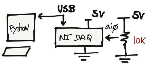
Start by including the nidaqmx library. Change the device_name variable according to the name of your device. Change ai0 to any other analog input that you would like to use.
import nidaqmx
from nidaqmx import constants

import time

device_name = "6001_Dev1/ai0"
There are a couple of ways to write this code using the nidaqmx python drivers. This can be confusing at first but hopefully the examples below can show the differences.
ai_single_demand_v1()
This version creates the analog task using the nidaqmx.Task() function. If you run this function, it will acquire N samples at Ts sampling time and prints the result on the terminal.
Note: Have in mind that this sampling time is not deterministic, and the acquisition of values might not be exactly Ts times apart.
def ai_single_demand_v1():
    #  Create Task
    analog_task = nidaqmx.Task()

    #  Create Virtual Channel - Analog Input
    analog_task.ai_channels.add_ai_voltage_chan(physical_channel=device_name,
                                                name_to_assign_to_channel="",
                                                terminal_config=constants.TerminalConfiguration.RSE,
                                                min_val=-10.0,
                                                max_val=10.0,
                                                units=constants.VoltageUnits.VOLTS,
                                                custom_scale_name=None)

    #  Start Task
    analog_task.start()

    #  Acquire Analog Value
    Ts = 1  # Sampling Time
    N = 5
    for k in range(N):
        value = analog_task.read()
        print(value)
        time.sleep(Ts)

    #  Stop and Clear Task
    analog_task.stop()
    analog_task.close()
When tasks are created by calling nidaqmx.Task(), you are responsible to clear and close the task whenever you are done. If you don't do that, it will generate a resource warning when the program is done.
ai_single_demand_v2()
If you use the with statement instead of the nidaqmx.Task() to create a task, then you don't need to worry about clear and closing the task at the end. The rest of the code is exactly the same as the previous one.
def ai_single_demand_v2():
    #  Create Task
    with nidaqmx.Task() as analog_task:

        #  Create Virtual Channel - Analog Input
        analog_task.ai_channels.add_ai_voltage_chan(physical_channel=device_name,
                                                    name_to_assign_to_channel="",
                                                    terminal_config=constants.TerminalConfiguration.RSE,
                                                    min_val=-10.0,
                                                    max_val=10.0,
                                                    units=constants.VoltageUnits.VOLTS,
                                                    custom_scale_name=None)

        #  Start Task
        analog_task.start()

        #  Acquire Analog Value
        Ts = 1  # Sampling Time
        N = 5
        for k in range(N):
            value = analog_task.read()
            print(value)
            time.sleep(Ts)

        #  Stop and Clear Task
        # no need to include because "with" takes care of it.
Analog Input - Virtual Channel Parameters
Change the parameters of the analog input virtual channel according to your application needs.
#  Create Virtual Channel - Analog Input
analog_task.ai_channels.add_ai_voltage_chan(
     physical_channel=device_name,
     name_to_assign_to_channel="",
     terminal_config=constants.TerminalConfiguration.RSE,
     min_val=-10.0,
     max_val=10.0,
     units=constants.VoltageUnits.VOLTS,
     custom_scale_name=None)
Call the desired function from the main function.
if __name__ == "__main__":
    # ai_single_demand_v1()
    ai_single_demand_v2()
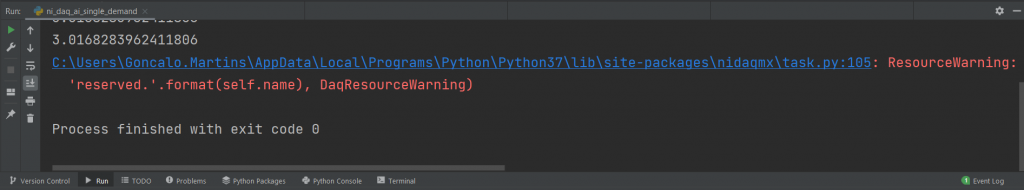
Result
This implementation works great if your goal is to visualize the analog input values not that often. The code is simple and easy to use.
Plot
Instead of printing the results on the terminal, we can render the values on a plot. There are several ways of plotting values in python, but I will cover the two most common ones: plots using matplotlib and plots using pyqtgraph. I recommend using pyqtgraph to plot graphs with real-time rendering requirements, however both ways can be integrated with GUIs.
Matplotlib Example
Start by including the required matplotlib and numpy libraries. Create some global variables that are related with the plotting. The NI task handler related to the analog_task is now a global variable too.
import nidaqmx
from nidaqmx import constants

import time

import matplotlib.pyplot as plt
import matplotlib.animation as animation
import numpy as np

device_name = "6001_Dev1/ai0"
analog_task = None

#  Create figure for plotting
fig = plt.figure()
ax = fig.add_subplot(1, 1, 1)
xs = []
ys = []
sample_index = 1
ai_single_demand_matplotlib()
This function is not much different that the functions described for the terminal code example. The main different is that the code that was under the Acquire Analog Value comment is going to be moved inside a function (animate function) that will plot the analog values at a certain interval.
The easiest way to make a live animation in Matplotlib is to use one of the Animation class. In this particular case we pass the animate function as the function to run as a live animation. You can adjust the interval parameter according to your needs.
def ai_single_demand_matplotlib():
    #  Create Task
    global analog_task
    with nidaqmx.Task() as analog_task:

        #  Create Virtual Channel - Analog Input
        analog_task.ai_channels.add_ai_voltage_chan(physical_channel=device_name,
                                                    name_to_assign_to_channel="",
                                                    terminal_config=constants.TerminalConfiguration.RSE,
                                                    min_val=-10.0,
                                                    max_val=10.0,
                                                    units=constants.VoltageUnits.VOLTS,
                                                    custom_scale_name=None)

        #  Start Task
        analog_task.start()

        #  Acquire Analog Value
        # Set up plot to call animate() function periodically
        global ax, xs, ys, fig
        ani = animation.FuncAnimation(fig, animate, fargs=(ax, xs, ys), interval=100)
        plt.show()

        #  Stop and Clear Task
        # no need to include because "with" takes care of it.
animate()
The animate function is responsible to acquire the data and plot it. You can adjust this function according to your plot needs too.
# This function is called periodically from FuncAnimation
def animate(i, ax, xs, ys):

    #  Acquire Analog Value
    global analog_task
    value = analog_task.read()

    # Add x and y to lists
    global sample_index
    sample_index = sample_index + 1
    xs.append(sample_index)
    ys.append(value)

    # Limit x and y lists to 20 items
    xs = xs[-20:]
    ys = ys[-20:]

    # Draw x and y lists
    ax.clear()
    ax.plot(xs, ys)

    # Format plot
    plt.ylim([-10.0, 10.0])
    plt.xticks(rotation=45, ha='right')
    plt.subplots_adjust(bottom=0.30)
    plt.title('Analog Voltage')
    plt.ylabel('Volts')
Call the ai_single_demand_matplotlib() from the main function.
if __name__ == "__main__":
    ai_single_demand_matplotlib()
Result

I connected a potentiometer to the analog input and vary the voltage so we can see the plot changing over time.
Pyqtgraph Example
One reason why pyqtgraph plots faster than matplotlib is because the underlying code of pyqtgraph is in C/C++ and the Python bindings are merely meant for invoking that code. The downside is that we need to write a bit more code to have the plots running.
In this case, we need to import the pyqtgraph library and some additional libraries (sys and deque).
import nidaqmx
from nidaqmx import constants

import pyqtgraph as pg
from pyqtgraph.Qt import QtGui, QtCore

import sys
from collections import deque

device_name = "6001_Dev1/ai0"
analog_task = None
ai_single_demand_pyqtgraph()
The code on this function is pretty much the same as the code for matplotlib. The main different is that we create the object Graph that will be responsible to plot the analog values instead of the animate function.
def ai_single_demand_pyqtgraph():
    #  Create Task
    global analog_task
    with nidaqmx.Task() as analog_task:

        #  Create Virtual Channel - Analog Input
        analog_task.ai_channels.add_ai_voltage_chan(physical_channel=device_name,
                                                    name_to_assign_to_channel="",
                                                    terminal_config=constants.TerminalConfiguration.RSE,
                                                    min_val=-10.0,
                                                    max_val=10.0,
                                                    units=constants.VoltageUnits.VOLTS,
                                                    custom_scale_name=None)

        #  Start Task
        analog_task.start()

        #  Acquire Analog Value
        q = Graph()

        #  Stop and Clear Task
        # no need to include because "with" takes care of it.
Class Graph
The class Graph uses Qt resources to plot the data. The update function is attached to a QTimer that it is called at regular intervals.
class Graph:
    def __init__(self, ):
        self.dat = deque()
        self.maxLen = 50  # max number of data points to show on graph
        self.app = QtGui.QApplication([])
        self.win = pg.GraphicsLayoutWidget()
        self.win.show()

        self.p1 = self.win.addPlot(colspan=2, title='Analog Voltage')
        self.p1.setYRange(-5.0, 5.0)
        self.curve1 = self.p1.plot()

        graphUpdateSpeedMs = 50
        timer = QtCore.QTimer()  # to create a thread that calls a function at intervals
        timer.timeout.connect(self.update)  # the update function keeps getting called at intervals
        timer.start(graphUpdateSpeedMs)
        sys.exit(self.app.exec())

    def update(self):
        if len(self.dat) > self.maxLen:
            self.dat.popleft()  # remove oldest

        global analog_task
        self.dat.append(analog_task.read())

        self.curve1.setData(self.dat)
        self.app.processEvents()
Call the ai_single_demand_pyqtgraph() from the main function.
if __name__ == "__main__":
    ai_single_demand_pyqtgraph()
Result
I used the same potentiometer on the analog input and vary the voltage so we can see the plot changing over time.
GUI
On this last visualization method I replicated Figure 1 using PyQt6 and Qt Creator. If you are not familiar how to create GUIs, I recommend reading [Ref 3] first.
To run this example, you need the ni_daq_ai_single_demand_gui.py and ni_max_onDemand.ui files available on the Python Files section.
Note: I am not including the icons for the start and stop button, sorry. If you run this example, those images are going to miss. Eventually I will include the PyCharm project with all those images.
I used a potentiometer on the analog input and vary the voltage so we can see the plot changing over time.
Code Diagrams
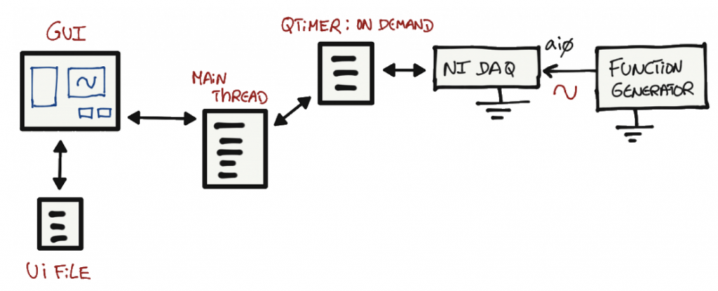
The goal with this section is to provide several different types of block diagrams that allow the understanding of the GUI code.
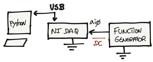
The first diagram is a generic block diagram on how the code, GUI, ui file and external hardware interact with each other in an conceptual way.
The second diagram was generated using code2flow and finds all function definitions in the code, and determines where those functions are called.

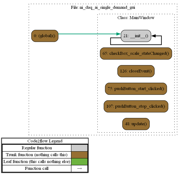
The above diagram provides a good estimate of the project’s overall structure.
When not to use it...
If your goal is to capture analog values where the sampling rate is important, you should avoid using the on demand mode.
We can do a simple test to understand the limitations of using on demand acquisition.
- On the pyqtgraph code the graph update speed is 50ms which in this case corresponds to a sampling frequency of 20Hz (Fs).
- For a decent time reconstruction of the signal in the time domain the maximum input frequency should be around Fs/10 = 2Hz.
Note: using Nyquist (Fs/2) will not be sufficient for a more detailed time analysis. You need more points if you want to analyze your data more accurately.
- If we connect a function generator to the analog input pin, and generate a sinusoidal waveform and change the frequency of the signal, we can start seeing the limitations of using on demand acquisition for signals that require a more rigid sampling time.
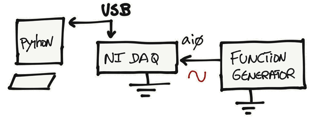
- Another challenge arises if we want to acquire faster signals. For an input signal of 1kHz, a good sampling frequency would be 10kHz (0.1ms). Good luck rendering that fast 🙂

We need to find another strategy to accommodate the acquisition of higher frequency signals meeting the desired sampling frequency. Check continuous and finite acquisition modes.
Python Files
References
- [Ref 1] “Plotting with Matplotlib”, pythonguis Website [Article]
- [Ref 2] Pyqtgraph examples -> run command: python3 -m pyqtgraph.examples
- [Ref 3] “Simple Qt GUI”, EngrEDU Glue Article [Article]
- [Ref 4] "Embedding custom widgets from Qt Designer" - pythonguis Website [Article]