
Formula DSP Algorithms
“Formula is a free and open-source integrated development environment to create your own audio effects the simplest way possible”.
This article shows how to use Formula and go from a DSP equation to a functioning implementation without involving any DSP theory.
Software Installation
Download Formula from soundspear website and follow the installation guidelines.
“Formula can either be used as an effect plugin inside your DAW (VST3 or AU), or as a standalone application. The effects within Formula are made using the C programming language”.
Then download and install the EQ Curve Analyzer plugin from Bertom Audio. This software “is an analyzer and signal generator plugin to see the frequency response (magnitude and phase) of any plugin or hardware”.
At last, I will be using Ableton as the DAW for the examples in this article but you can use any other DAW of your choice.
DAW Setup
Open your DAW and in an audio track add two instances of the EQ Curve and the Formula Plugin in between them.
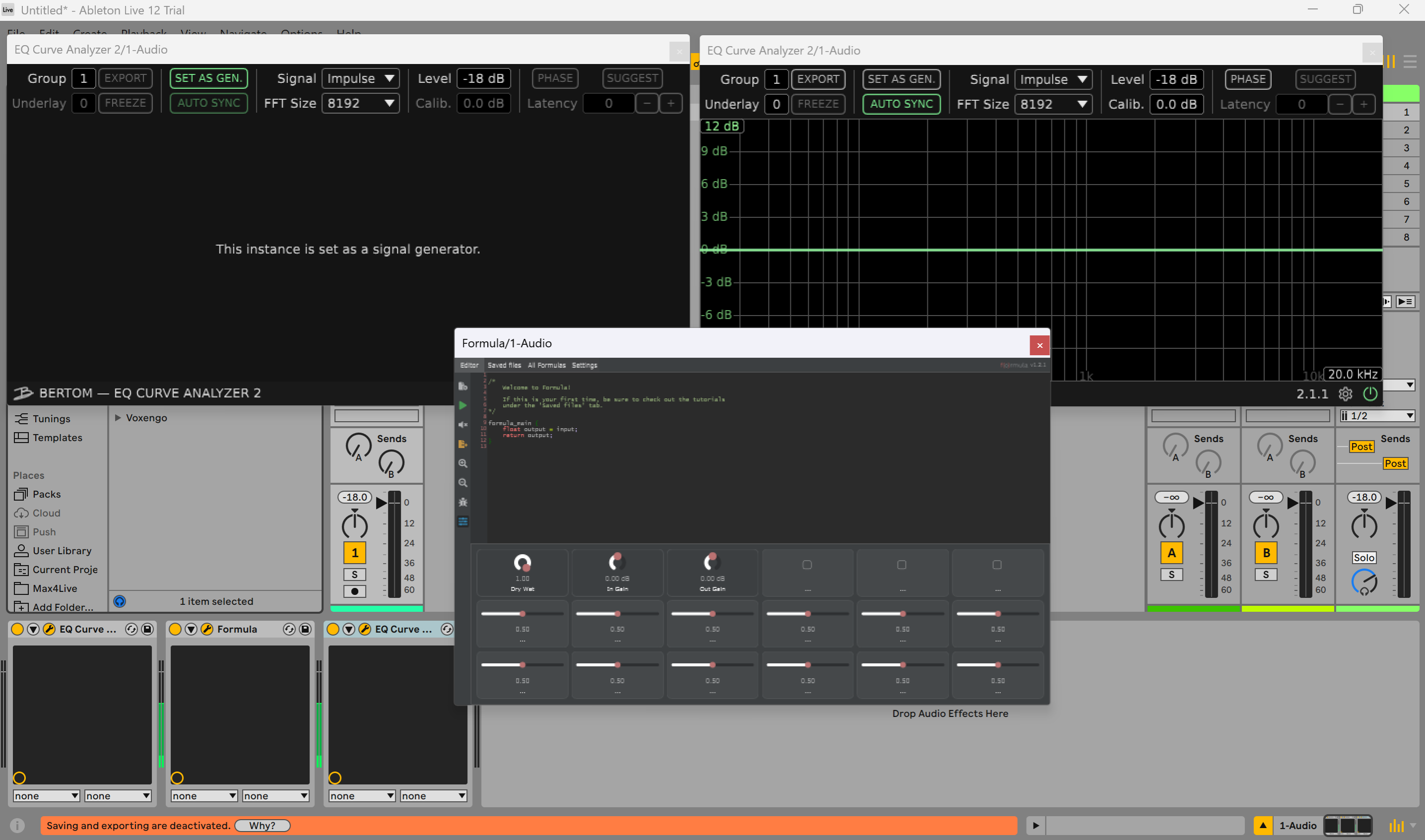
The first EQ Curve is a signal generator, that will generate an impulse signal that will go through the Formula plugin. The Formula plugin is then connected to a second instance of an EQ Curve that is set to plot the magnitude and phase response of the signal.
I know I said no theory, but I can’t resist to show the connection with some graphs and jargon that you typically see in DSP or control theory books about the impulse response of a system with the DAW plugins.
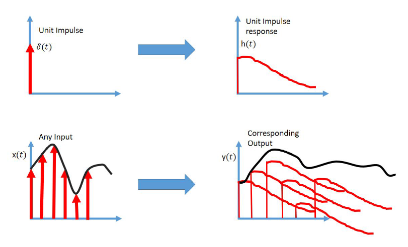
The first EQ Curve plugin is generating the impulses (red arrows pointing up), that stimulate the system (Formula Plugin), that has a response (black curve) that get displayed on the second EQ Curve plugin 😌
Anyway… if this seems to abstract to digest don’t worry too much about it. This is just showing the importance of the impulse signal in characterizing the response of a system.
First Formula Code
Before starting this section, I recommend downloading and reading the Formula user manual. It is very well done, simple to read and gives you a good foundation to start using the plugin.
The first example that I like to show is a simple gain knob that controls the volume of the input signal.
formula_main {
    float gain = KNOB_1;

    float output = input * gain;

    return output;
}
If you run this code and move the gain knob up and down, you can see in the frequency response the gain moving up and down accordingly.
1st Order Analog Low Pass Filter (IIR type)
Believe it or not but we are in good shape to start implementing some filters and see the frequency response in real-time.
I am going to use the book “Designing Audio Effect Plugins in C++: For AAX, AU, and VST 3 with DSP Theory”, by Will Pirkle. It has plenty of examples ready to use that we can test with this setup.
I am going to start with a simple first order analog RC filter (IIR type) on page 266, 267, and 268.
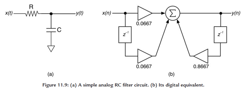
Figure 11.9, shows the analog filter and respective digital implementation. I am going to skip the math in this article just to make it simpler to follow the rest of the text. Briefly, the coefficients of the digital implementation were calculated to have a cut-off frequency at 1kHz at a 44.1kHz of sampling rate.
With that we have the following difference equation:
y(n)=0.0667\;x(n) + 0.0667 \; x(n-1) + 0.8667 \; y(n-1)
Let’s program this in Formula:
// State variables
float x_n, x_n1, y_n, y_n1;

formula_main {

    // Get Input Samples
    x_n = input;

    // Computer Filter
    y_n = 0.0667 * x_n + 0.0667 * x_n1 + 0.8667 * y_n1;

    // Update States
    x_n1 = x_n;
    y_n1 = y_n;

    return y_n;
}
Run the code and you will see the filter response.
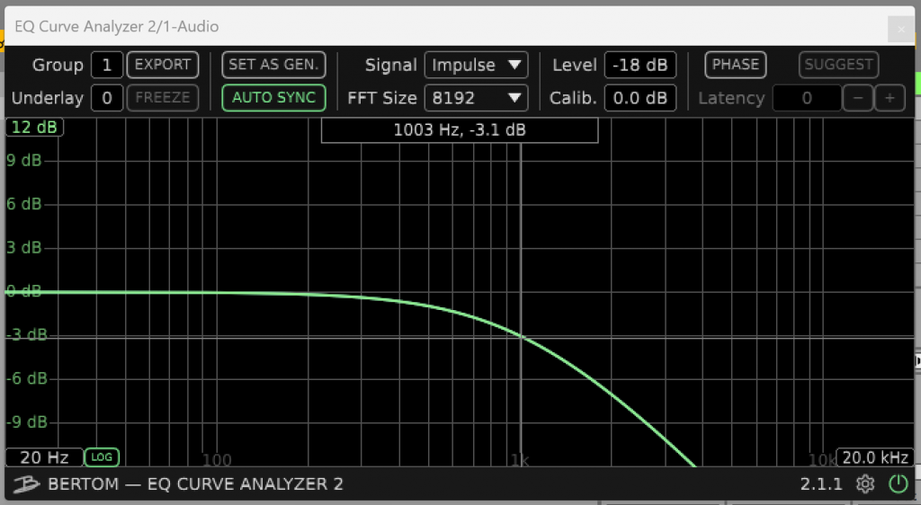
Notice the -3 dB gain at the 1kHz cut-off frequency.
Pretty cool 😊
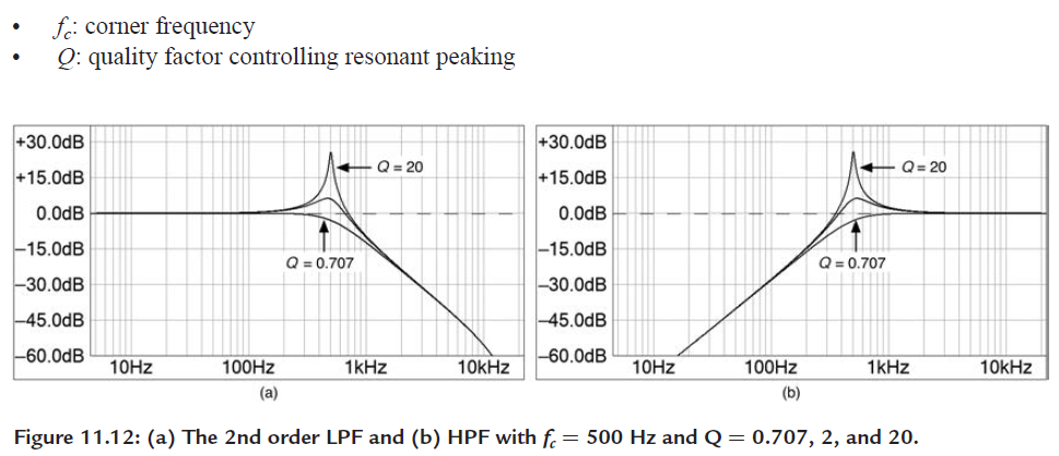
2nd Order Filter with Q factor
Let’s ramp up the difficulty of our Formula code a bit and include a knob that controls the quality factor (Q – resonant peak) and the cut-off frequency of a 2nd order low pass filter (from page 271 and 272).
We will be using a biquad filter structure in direct form:
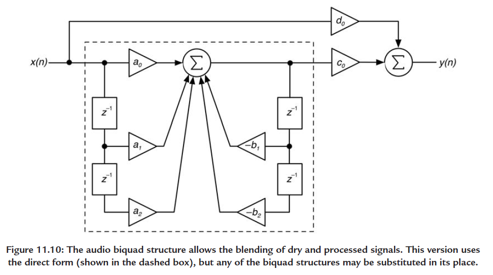
That has the following difference equation:
y(n)= d_0 \; x(n) + c_0 \; (a_0 \; x(n) + a_1 \; x(n-1) + a_2 \; x(n-2) \\ - b_1 \; y(n-1) - b_2 \; y(n-2))
The code is a bit more extensive but not much different from the code that we have been doing.
// State variables
float x_n, x_n1, x_n2, y_n, y_n1, y_n2;
formula_main {
// Filter Parameters and Respective Knobs
float fc = 200 + (KNOB_1 * 20000);
float Q = (KNOB_2 * 20) + 0.707;
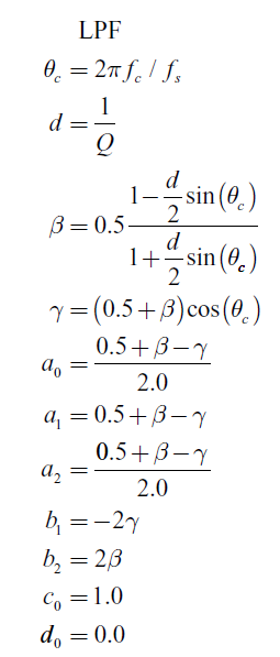
float theta_c = 2 * M_PI * fc / SAMPLE_RATE;
float d = 1.0 / Q;
float beta = 0.5 * ((1.0 - (d/2)*sin(theta_c)) / (1.0 + (d/2)*sin(theta_c)));
float gamma = (0.5 + beta)*cos(theta_c);
// Coefficients
float a0 = (0.5 + beta - gamma)/2.0;
float a1 = 0.5 + beta - gamma;
float a2 = (0.5 + beta - gamma)/2.0;
float b1 = -2.0 * gamma;
float b2 = 2.0 * beta;
// Dry/Wet and filter output gain control
float d0 = 0.0;
float c0 = 1.0;
// Get Input Sample
x_n = input;
// Computer Filter
y_n = d0 * x_n + c0 * ( a0*x_n + a1*x_n1 - b1*y_n1 - b2*y_n2 );
// Update States
x_n2 = x_n1;
x_n1 = x_n;
y_n2 = y_n1;
y_n1 = y_n;
return y_n;
}
Hope this helps understanding how to implement DSP filters with Formula. Go ahead and try other filters and effects from the book or other sources and have fun 😎
References
- [Ref 1] “Formula VST”, soundspear.com [Website]
- [Ref 2] “Bertom Audio”, bertomaudio.com [Website]
- [Ref 3] “Designing Audio Effect Plugins in C++: For AAX, AU, and VST 3 with DSP Theory”, by Will Pirkle [Book]